4. Internal Convergence and China’s Growth Potential

Yang Yao and Mengqi Wang

Introduction

Amid declining growth rates, the debate about China’s growth potential has re-emerged. Something overlooked in this debate, however, is the role played by internal convergence. China’s unprecedented growth over the past 30 years or so, and particularly in the years before the Global Financial Crisis (GFC), has been concentrated in its coastal provinces, while the vast inland areas have largely lagged behind. By 2015, per capita gross domestic product (GDP) in the eastern provinces was 1.8 times that in the central and western regions. Shanghai, the richest province in China, enjoyed a per capita GDP of $15,265 in 2015, 3.5 times that of Guizhou, one of the poorest provinces in China. Since the GFC, growth in the eastern provinces has slowed, while growth in the inland provinces has picked up. Internal convergence could serve as a driver for the growth of China’s inland provinces.

This chapter studies how internal convergence can contribute to China’s long-run growth. In particular, we study three kinds of convergence: regional, efficiency and technological. Regional convergence is the convergence of provinces within China’s eastern (coastal), central (inland) and western (inland) regions, and allows China’s inland provinces to enjoy the advantage of backwardness to sustain a longer period of high-speed growth. Efficiency convergence is the convergence of the two inland regions towards the efficiency level maintained by the eastern region, and pulls inland provinces to the production frontier, so the growth rates in their transition paths become higher. Technological convergence is the convergence of the two inland regions towards the speed of technological progress achieved by the eastern region, and raises the inland regions’ steady-state growth rates. Technological convergence also increases inland regions’ growth rates in their transition paths because the steady-state growth rate is part of the growth rate in the transition path. The three kinds of convergence thus have the potential to greatly enhance China’s overall long-term growth.

Our analysis is organised as follows. In the next section, we introduce the theoretical framework of our analysis, which is based on the neoclassical growth model and China’s regional growth disparities. In section three, we introduce the data and correction methods to the growth figures reported for various provinces. In section four, we estimate the growth equations for each region and nationally and, in section five, we present our forecast for the growth potential of each region and for the country as a whole. Using that forecast, we then conduct several policy experiments as well as a counterfactual analysis to study the effects of the three kinds of convergence. Section six concludes the chapter.

The theoretical framework

The theoretical basis for the three types of convergence studied in this chapter is neoclassical growth theory. It is well known that the theory predicts conditional convergence among countries or regions (Barro and Sala-i-Martin 1992). Specifically, since countries/regions have a steady state (where growth in per capita GDP is the rate of technological progress), countries/regions with lower levels of per capita GDP (or lower levels of capital stock) should grow faster than those with higher levels of per capita GDP (or higher levels of capital stock). Ultimately, therefore, per capita GDP converges (σ-convergence).

In reality, countries/regions may not have the same steady state, in terms of having the same rates of saving and technological progress in particular. Thus, income convergence is not realised. However, given its own steady-state growth rate, a country/region nonetheless grows faster when its per capita GDP is low than when its per capita GDP becomes higher (so-called β-convergence). This provides the basis for the advantage of backwardness, which, in turn, forms the basis of the first kind of convergence to be examined in this chapter: regional convergence.

In the past 20 years, China’s growth has been concentrated in its coastal provinces (the eastern region), while the two inland areas lagged behind. The reasons for this include the fact that the eastern region: 1) maintains a higher level of resource efficiency; and 2) has faster rates of technological progress. Eastern provinces are now close to their steady states, so their growth rates have declined. Inland provinces, however, remain at a distance from their steady states, so their growth rates, at least theoretically, can be high relative to those of the eastern region. If the inland regions can realise higher growth rates, the country as a whole can maintain a higher growth rate.

The second type of convergence sees inland regions obtaining the investment efficiency of the eastern region, and the third type sees them reaching the technological progress levels of the east. To provide a more structured view of the three types of convergence, let us consider the following variant of the Solow model with technological progress.

Let a region’s production function be expressed by Equation 4.1.

Equation 4.1

Y = (Kδ)^a(AL)^1–a, 0 < a < 1

In Equation 4.1, K captures the stock of capital, L is the stock of labour (population), Y is output and a is the output elasticity of capital (so 1–a is the output elasticity of labour). In addition, δ is an index of the efficiency of capital utilisation and A is an index of a labour-augmenting technology. The efficiency of capital utilisation is constant and A grows at a constant rate, η. The population grows at a constant rate of n. L^* = AL is the stock of effective labour, which has a growth rate of . Output per effective labour is shown as Equation 4.2.

Equation 4.2

Output per labour unit is therefore y = Ay^*, and we can now show that in the transition path the growth rate of output per effective labour is shown as Equation 4.3.

Equation 4.3

In Equation 4.3, k = K/L is capital stock per unit of labour, so the growth rate of output per labour unit (or GDP per capita) in the transition path is shown as Equation 4.4.

Equation 4.4

In other words, the growth of GDP per capita in the transition path is derived from two sources. First—represented by the terms in the right-hand bracket—is growth of capital stock per capita adjusted by the efficiency of capital utilisation. Second, is the growth of the labour-augmenting technology, the rate of which is η. The two sources are weighted by the output elasticities of capital and labour, respectively.

In the steady state, output per effective labour becomes constant. By Equation 4.3, we get Equation 4.5.

Equation 4.5

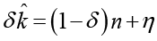
From Equation 4.5, we in turn obtain the growth rate of GDP per capita in the steady state (Equation 4.6).

Equation 4.6

That is, the growth rate of GDP per capita at the steady state is equal to the rate of technological progress. This is the standard result of the Solow model for technological progress.

The above model informs our understanding of the three kinds of convergence we have defined. First, Equation 4.5 implies β-convergence: when per capita GDP is low, the rate of growth of per capita capital stock, , is large,¹ as is the rate of growth of per capita GDP. This is what we refer to as regional convergence. The two inland regions still have low per capita GDP, meaning their growth rates should be higher when they follow their own rates of convergence than when they follow the national rate of convergence. In other words, regional (club) convergence could help China maintain a higher growth period for longer.

Second, Equation 4.5 also explains the second kind of convergence. The equation informs us that a higher efficiency index, d, increases the growth rate of GDP per capita. To the extent that the eastern region has the highest level of investment efficiency, convergence of the two inland regions towards that level will increase their growth rates. The national growth rate will, in turn, also rise. Last, Equations 4.5 and 4.6 tell us that a higher rate of technological progress boosts the growth rate of per capita GDP in the steady state as well as in the transition path. Again, because the eastern region has the highest rate of technological progress, convergence of the two inland regions towards the rate of the eastern region will increase not only their own growth rates, but also the national growth rate.

Data

Data used in this study include real GDP per capita and its growth rate, alongside the growth rate of real investment per capita across 28 provinces² in China and over the period 1984–2015. We collect the data from China Statistics Yearbooks (NBS 1985–2016) and The Gross Domestic Product of China: 1952–1995 (NBS 1997).

One issue when using provincial GDP data is a tendency by local governments to overstate growth rates. It is widely acknowledged that the published growth rates of almost all provinces in China have been consistently higher than the published national growth rate. To account for this, we adopt a method of deflation to correct provincial growth rates as follows.

First, we calculate the national average growth rate of real GDP among all provinces for each year, weighted by their shares of real GDP in the national total. Second, to obtain the deflator for each year, we divide this average growth rate by the national growth rate as published by the National Bureau of Statistics of China (NBS). Third, we deflate each province’s growth rate in any particular year by the common deflator for that year. Fourth, assuming that the GDP figures of the base year (1984) were not inflated, we then apply the deflated growth rates to capture the ‘true’ GDP figures for each year thereafter. Finally, by dividing the deflated GDP by each province’s population, we get each province’s per capita GDP for each year.

Our study involves estimation of the growth equation, during which we will study only one input: the real growth rate of investment per capita. Since the NBS publishes only nominal figures of investment, we obtain the real growth rates of investment by deflating the value of investment by the price indices of fixed investment. Depreciation rates for investment after 1995 are from the China Statistics Yearbooks (NBS 1985–2016) and those before 1995 are constructed according to Zhang et al. (2004) and using investment data from The Gross Domestic Product of China: 1952–1995 (NBS 1997).

The 28 provinces are divided into three regions: eastern, central and western.³ Summary statistics of the main variables by region are presented in Table 4.1. The national data are simple averages of the 28 provinces.

Table 4.1 Summary statistics

	Real GDP per capita (RMB100)	Growth rate of real GDP per capita	Growth rate of real investment per capita
Panel A: Eastern
Observations	288	288	288
Mean	49.497	0.085	0.127
Std deviation	45.758	0.049	0.141
Maximum	243.329	0.227	1.384
Minimum	4.700	–0.110	–0.244
Panel B: Central
Observations	320	320	320
Mean	23.523	0.086	0.127
Std deviation	20.367	0.038	0.138
Maximum	114.853	0.198	0.973
Minimum	2.985	–0.043	–0.370
Panel C: Western
Observations	288	288	288
Mean	18.848	0.084	0.135
Std deviation	15.989	0.062	0.147
Maximum	87.995	0.555	0.729
Minimum	2.683	–0.347	–0.288
Panel D: National
Observations	896	896	896
Mean	30.369	0.085	0.130
Std deviation	32.840	0.050	0.142
Maximum	243.329	0.555	1.384
Minimum	2.683	–0.347	–0.370

Notes: The period covered is 1984–2015. Tibet, Hainan and Chongqing are not included due to missing data. GDP and its growth rates are modified under the assumption that the national figures reported by the NBS are correct.

Source: Original data are from NBS (1985–2016).

Figure 4.1 shows the growth of GDP per capita in each region using the modified GDP data. On average, the eastern region has grown faster than the two other regions. As a result, the economies of the country’s coastal provinces and those of its inland provinces have diverged. The gap between the central region and the western region has also grown over the years. By 2015, the per capita GDP of the eastern region was two times that of the central region, while per capita GDP in the western region was 23 per cent lower than in the central region. These contrasts provide the basis for this study. Since the gap is greatest between the eastern region and the other two regions, we will study the catch-up process of the two inland regions.

Figure 4.2 presents each region’s average growth rate of real GDP per capita and Figure 4.3 shows the average growth rate of real investment per capita for each region over the period 1984–2015. The eastern region led the growth of real GDP until 2007, after which it was overtaken by the two inland regions. The eastern region had higher rates of investment growth than the two inland regions until the middle of the 1990s, but much lower rates since 2000. Clearly, investment efficiency has been lower in the two inland regions, particularly across China’s high-growth period of 2001–08. This provides the basis for the potential internal convergence of efficiency.

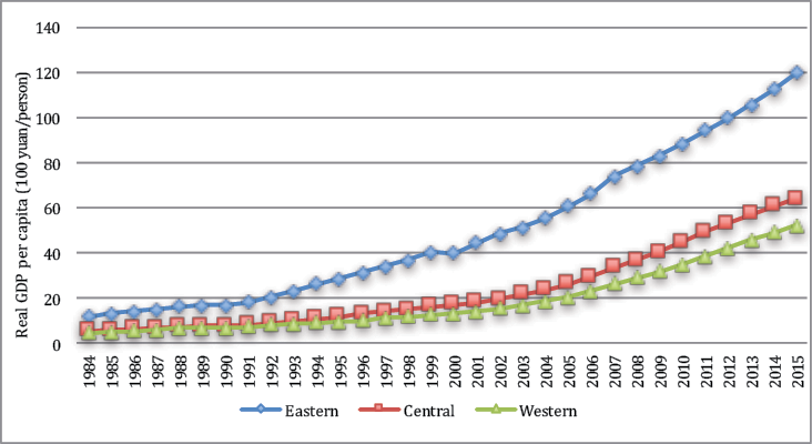
Figure 4.1 Real GDP per capita (RMB100 per capita)

Note: GDP per capita is measured in 1984 renminbi and is adjusted under the assumption that the national growth rates published by the NBS are correct.

Source: Original data from NBS (1985–2016).

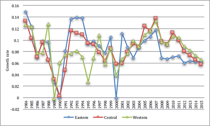
Figure 4.2 Growth rates of real GDP per capita

Note: The growth rates presented are adjusted under the assumption that the national growth rates published by the NBS are correct.

Source: Original data from NBS (1985–2016).

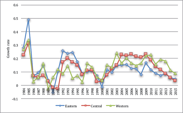
Figure 4.3 Growth rates of real investment per capita

Source: The growth rates of real investment are obtained by applying the price indices of fixed investment to the nominal investment data published by NBS (1996–2016). The price indices before 1995 are constructed according to Zhang et al. (2004) using investment data from NBS (1997).

Estimation of the growth equations

Econometric setups

We estimate two growth equations: one to determine the conditional convergence of each region and the other to determine the conditional convergence of the whole country. Both are consistent with the theoretical model introduced in the previous section. The first equation assumes heterogeneous parameters for individual regions and takes the following specification (Equation 4.7).

Equation 4.7

In Equation 4.7, the dependent variable g_it is the modified annual growth rate of real GDP per capita for province i in year t. On the right-hand side, ln(y_i,t–1) is log-lagged real GDP per capita, which aims to capture the convergence effect. We allow for different speeds of convergence in different regions. D_C and D_W are two dummy variables representing the central and western regions, respectively. As a result, β_E measures the speed of convergence in the eastern region and β_E+β_C and β_E +β_W measure, respectively, the speeds of convergence in the central and western regions. Next, G_it is the growth rate of real investment per capita in province i in year t. To capture the different levels of efficiency in individual regions, we estimate a different coefficient for G_it for each region. We expect that δ_E, the efficiency coefficient for the eastern region, is larger than that for the other two regions—that is, δ_C and δ_W should be negative. To measure the rate of technological progress in each region, we estimate a linear time trend for each. The parameters η_E, η_E + η_C and η_E + η_W are, respectively, the speeds of technological progress in the eastern, central and western regions. We expect that η_E is positive and the other two parameters, η_C and η_W, are negative. We also add province fixed effects to control the influences of unobserved province-specific and time-invariant factors. Last, ε_it is an independent and identically distributed (IID) error term.

By Equation 4.7, we can calculate the steady-state growth rate for each region. In the steady state, the growth rate of investment per capita is constant, as is the growth rate of GDP per capita. So, for any two consecutive periods, t and t – 1, we have the following (Equation 4.8).

Equation 4.8

In Equation 4.8, represents the estimates for β_E, β_E + β_C and β_E + β_W and represents the estimates for η_E, η_E + η_C and η_E + η_W. As a result, the steady-state growth rate, which equals ln(y_j,t) – ln (y_j,t–1), is shown as Equation 4.9.

Equation 4.9

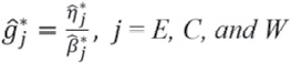
This, of course, is a restatement of a result derived by the neoclassical growth model: the growth rate of GDP per capita in the steady state is equal to the long-term speed of technological progress.

To study convergence nationally, we estimate the following common-parameter equation (Equation 4.10).

Equation 4.10

g_it = α + βln(y_i,t–1) + δG_it + η(t – 1983) + ϕ_i + ε_it

In this specification, we assume common speeds of convergence, efficiency of investment and technological progress in all provinces.

Estimation results

We report the results of Equations 4.7 and 4.10 in Table 4.2. The first three columns show the estimated parameters for each of the three regions in the heterogeneous-parameter specification. The speeds of convergence in the eastern, central and western regions are, respectively, 8 per cent, 7.1 per cent and 7.7 per cent. The eastern region converges the fastest because it has the highest per capita GDP and is therefore closer to its steady state than the other two regions. It is interesting, however, to find that the western region has a higher speed of convergence than the central region. The western region has a lower per capita GDP than the central region at the moment, so it must also have a lower per capita GDP than the central region in the steady state. This is one piece of evidence that the western region has impediments to its long-term technological progress.

Table 4.2 Regression results

	Eastern	Central	Western	National
Ln(lagged real GDP per capita)	–0.080***	–0.071***	–0.077*	–0.076***
	(0.015)	(0.021)	(0.044)	(0.016)
Investment growth	0.160***	0.141***	0.157***	0.154***
	(0.047)	(0.020)	(0.032)	(0.019)
Time trend	0.00613***	0.00606***	0.00601*	0.00606***
	(0.00127)	(0.00181)	(0.00327)	(0.00129)
Steady-state growth rate	7.66%	8.54%	7.81%	7.97%
Average province fixed effect	–0.020	–0.089	–0.092	–0.056
Constant	0.270***	0.270***	0.270***	0.239***
	(0.043)	(0.043)	(0.043)	(0.041)
Province FEs	Yes	Yes	Yes	Yes
R-squared	0.300	0.300	0.300	0.297
Observations	896	896	896	896

^* significant at 10 per cent

^** significant at 5 per cent

^*** significant at 1 per cent

Notes: This table shows the regression results of Equations 4.1 and 4.3. Columns 1–3 are results from Equation 4.1. Parameters are consolidated for the regions. Column 4 presents the results from Equation 4.4.

A 1 percentage point increase in the rate of investment growth can bring increases in the GDP growth rate of 0.16 percentage point for the eastern region, 0.141 for the central region and 0.157 for the west. As expected, the eastern region has the highest level of investment efficiency, while the level of investment efficiency in the western region is higher than in the central region. Technological progress in the eastern region is the fastest, growing at 0.613 per cent each year, followed by the central region on 0.606 per cent and the western region on 0.601 per cent. Based on Equation 4.3, we calculate the growth rate for each region in their respective steady states and present them in Table 4.2. We find that in their steady states, the eastern region would grow at 7.66 per cent, the central region at 8.54 per cent and the west at 7.81 per cent. These rates are high, for which we can see two reasons: the first is that the period studied was one of very high growth; and second is Chinese provinces are, on average, likely still far from reaching their steady states. Both of these factors can inflate the estimates of technological progress. As it is not the purpose of this chapter to make a forecast of China’s growth prospects, but rather to study how internal convergence raises China’s growth potential, attention should be paid to comparisons between different scenarios of convergence and not the growth rate levels.

The last column of Table 4.2 presents the regression results of Equation 4.4 for the national average. The speed of convergence is 7.6 per cent per annum, which is within the range obtained for the three regions. The rate of investment contribution is 0.154, which is also within the range obtained for the three regions. Finally, the speed of technological progress is 0.606 per cent, which is the same as that for the central region. Because the rate of convergence is higher nationally than in the central region, national growth in the steady state ends lower, at 7.97 per cent.

Forecast and analysis

With the estimation results in Table 4.2, we proceed to offer a forecast for China’s growth potential in the period 2016–30. Our focus is not the forecast itself, but analysis of the effects of internal convergence. Specifically, we study three kinds of convergence: 1) the two inland regions converge to their own steady-state growth rate with the speed of convergence of the eastern region; 2) the two inland regions reach the investment efficiency of the eastern region; and 3) the two inland regions reach the speed of technological progress of the eastern region. Because the eastern region has faster convergence than the other two regions, regional convergence would lower the GDP growth rates of the other two regions. This counterfactual analysis thus shows that the backwardness of the two inland regions actually offers the potential for China to sustain higher rates of growth into the future. The second kind of convergence helps the inland regions reach the efficiency frontier maintained by the eastern region. As a result, it increases the inland regions’ growth rates in their transition paths towards steady states. Last, the third kind of convergence raises the rates of the inland regions’ long-term technological progress to the level of the eastern region so they would have higher GDP growth rates in their steady states.

The steady-state growth rates of the three regions and the whole country were presented in Table 4.2. Our forecasting task is to estimate the GDP growth rates in the transition pathways. For region j, we use the following equation to iterate our forecast, starting in 2016 (Equation 4.11).

Equation 4.11

In Equation 4.11, the variables with the bars are the averages for the given region, and the key is to forecast the average growth rate of investment.

Forecasting investment growth

China has broadly followed a unique path of high savings and high investment since the People’s Republic was established in 1949. But in the decade leading up to 2012, the saving and investment rates were particularly high, reaching above 50 per cent of GDP. Although in the past several years the economy has embarked on a path of rebalancing, China’s saving and investment rates are still high by international standards. This makes it difficult to use an international benchmark to forecast China’s future investment growth. In this chapter, we adopt the time-series analysis model ARIMA (2, 2) to forecast China’s investment growth rates for the period 2016–30. Once again, our focus is not on the levels forecast; rather, the forecast offers a basis for us to study the effects of the three convergence types.

Our forecast adopts 2015 as the base year. Based on the observed investment growth rates in the period 1984–2015, we apply the ARIMA (2, 2) model to predict the investment growth rates of each region across the period 2016–30. The national forecast for each year is the weighted average of the three regions. Forecast per capita investment growth rates are presented in Figures 4.4a–d, alongside greater details listed in Appendix Table 4.A1. In all three regions, investment growth is predicted to pick up from 2016, but this is not what is observed that year.

Investment growth continued to decline in 2016. Again, however, our primary purpose is not to obtain exact estimates for the levels of investment growth; rather, we are more concerned with how improvements in investment efficiency would sustain higher growth rates in China. The future growth rates of investment in the eastern region are predicted to converge to 11.7 per cent from 2022. In the central region, investment growth will converge to 10.9 per cent from 2027. In the western region, investment has grown by very high rates in recent years, but it is expected to quickly converge to 12.8 per cent from 2021.

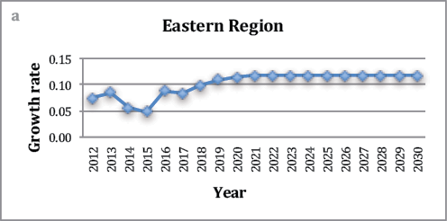
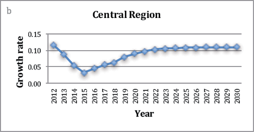
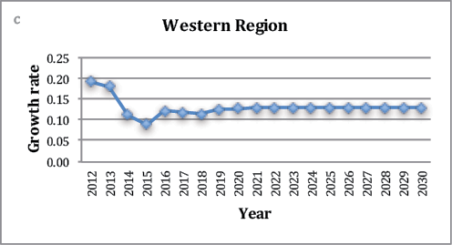
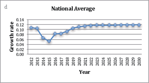
Figures 4.4a–d Forecast investment growth rates

Note: The forecast for each region is done using ARIMA (2, 2) based on the data for the period 1984–2015. The national average is the weighted average of the three regions’ growth rates.

Source: Authors’ calculation.

Forecasting GDP growth

Based on the forecast investment growth rates and applying Equation 4.11, we can forecast future growth rates of GDP per capita for each region. We can then compute the national weighted average growth rates.⁴ These forecasts are presented in Figures 4.5a–d together with their corresponding historical records. Detailed numbers are presented in Appendix Table 4.A2. In sum, all three regions see rising GDP growth rates over the coming decade—mostly brought about by the predicted higher investment growth rates in the ensuing few years and the positive speed of technological progress, as reported in Table 4.2. By 2025, however, growth rates for the three regions will have stabilised,⁵ although they will still be higher than in their respective steady states. That is, convergence towards the steady state will not begin in the 2016–30 period.

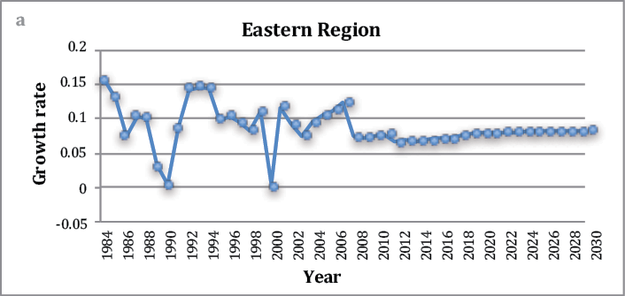
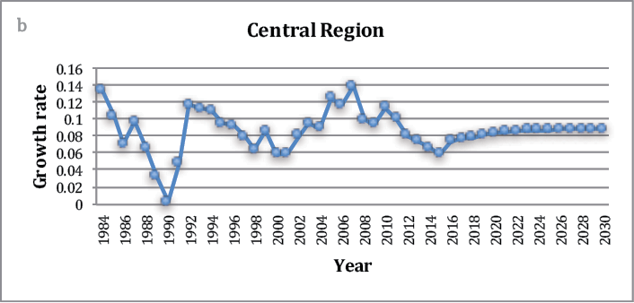
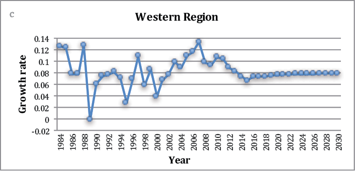
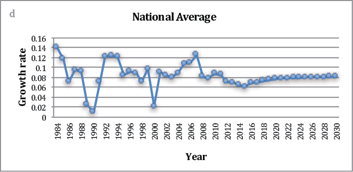
Figures 4.5a–d Forecast growth rates of GDP per capita

Note: The forecasts are done following Equation 4.11 and the forecast investment growth rates reported in Figure 4.4.

Source: Authors’ calculation.

Comparative analyses

As we have emphasised, our main purpose is to study the effects of the three kinds of convergence, which we will do in this subsection. Before this, however, we show that ignoring regional convergence could lead to underestimation of national growth potential. It amounts to making a comparison between the national growth rates calculated as the weighted averages of the forecast regional growth rates introduced above and the counterfactual in which the national growth rates are forecast by the estimated results of the national growth equation (Equation 4.10), the results of which are presented in the last column of Table 4.2.

Equation 4.10 assumes that all provinces share the same speed of convergence, have the same level of investment efficiency and converge to the same steady state. Subsequently, we will call estimates derived using Equation 4.10 ‘common-parameter estimates’. These form the counterfactual because, in reality, provinces in the three regions converge to different steady states at different speeds and have different levels of efficiency. Depending on the composition of those factors, the national growth rates calculated by the weighted averages of the three regions’ growth rates can be higher than the national growth rates forecast by the common-parameter estimates. Figure 4.6 shows that this is indeed the case here. The weighted-average forecast is 1.51 percentage points higher than the common-parameter forecast. In other words, this illustrates that ignoring regional convergence can lead to underestimation of the national growth potential. There are probably two explanations for this. First, the eastern region is more efficient and has a higher steady-state growth rate than the other two regions. In the meantime, its share of national GDP is also large (about 60 per cent). Second, the two inland provinces have slower convergence than the eastern region, meaning their high growth can be sustained for a longer period.

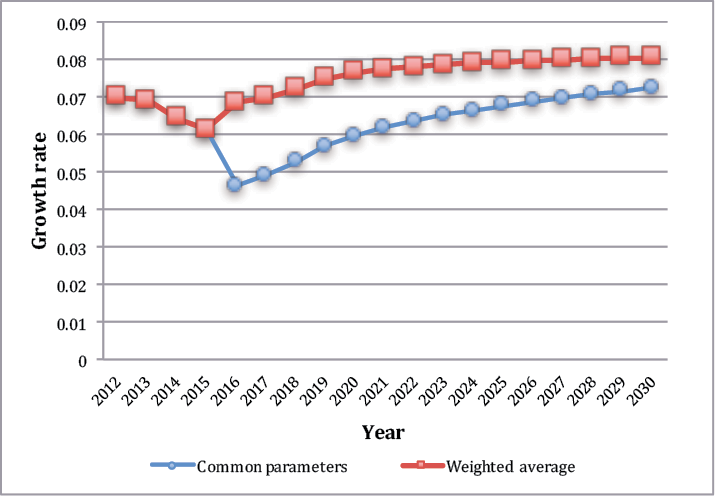
Figure 4.6 Common-parameter estimation versus heterogeneous-parameter estimation

Note: The common-parameter forecast uses the results of the national regression reported in Table 4.2 and the national investment growth rates forecast by the weighted averages of the three regions.

Source: Authors’ calculation.

We now study the effects of the first kind of convergence: regional convergence. We compare the central and western regions’ growth rates forecast by their respective growth equations with their growth rates in the counterfactual in which their speed of convergence catches up with the speed of convergence in the eastern region. The results are presented in Figures 4.7a–c, which also present a comparison with the national average. As expected, reaching the eastern region’s speed of convergence would lower the growth rates in the central and western regions. This is more the case in the central region than in the west because the central region has the lowest speed of convergence (Table 4.2). On average, the central region’s growth would slow by 2.7 per cent, while the western region’s growth would slow by only 0.8 per cent. Together, this would lead to an average reduction of 0.9 per cent in the national growth rate, which is equal to 11.7 per cent of the average national growth rate of 7.7 per cent that was originally forecast for the period 2016–30. In other words, the lower speeds of convergence in the two inland regions that result from the advantage of backwardness can indeed sustain higher national growth rates in China.

Coming to the effects of convergence on investment efficiency, we find these are very small—mostly because the coefficients of investment growth for the three regions (Table 4.2) do not differ much. On average, the growth rate in the central region would be increased by only 0.1 percentage points if the region’s investment efficiency caught up with that of the eastern region. In addition, the investment growth rate in the western region would stabilise at a higher rate than that of the eastern region, which would cancel the efficiency gains of the latter. As a result, the growth rates of the western region would be almost unchanged if it obtained the investment efficiency of the east.

Last, we study the effects of the convergence of technological progress. Technological progress has cumulative effects on the growth rate in the transition path, so convergence towards the level of technological progress in the eastern region would allow the other two regions to have substantially higher rates of growth in their transition path (although Table 4.2 shows that the eastern region does not lead the other two regions by large margins). Figures 4.8a–c illustrate these results, including that the improvements in technological progress are substantial. On average, the central region would grow 4.7 percentage points faster and the west 4.8 percentage points. As a result, the national economy would grow an average of 2.6 percentage points faster. This is more than one-third of the average national growth rate originally forecast for the period 2016–30. Therefore, convergence of technological progress has by far the largest effect of the three kinds of convergence on regional and national growth.

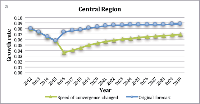
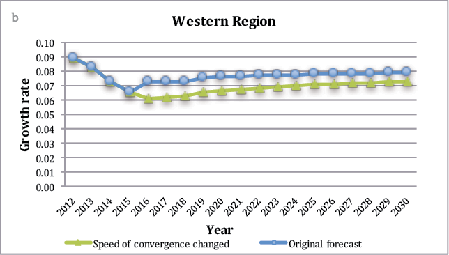
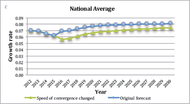
Figures 4.7a–c Effects of regional convergence

Notes: Original forecasts are the same as those presented in Figures 4.5a–d. The counterfactual forecasts assume that the central and western regions adopt the speed of convergence of the eastern region.

Source: Authors’ calculation.

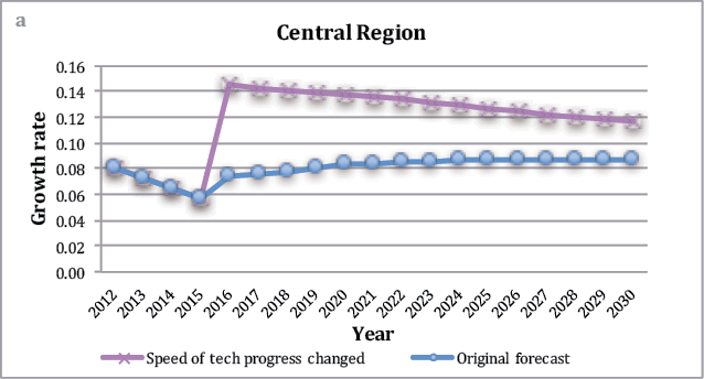
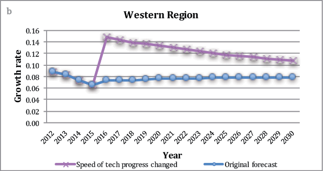
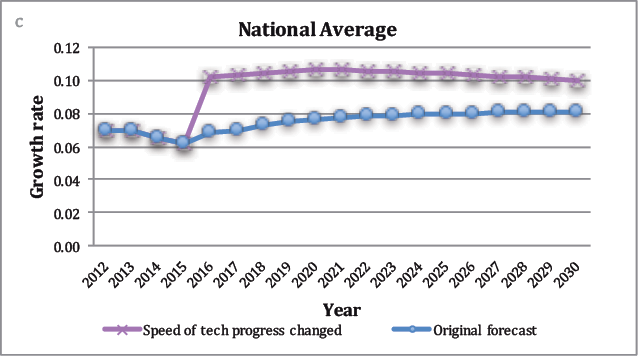
Figures 4.8a–c Effects of the convergence of technological progress

Note: Original forecasts are the same as those presented in Figure 4.5; the counterfactual forecasts assume that the central and western regions adopt the speed of technological progress of the eastern region.

Source: Authors’ calculation.

Conclusion

In this chapter, we have estimated growth equations for China’s three geographic regions and for the whole country. We have found different speeds of regional convergence, different levels of investment efficiency and different speeds of technological progress in the three regions, which provide the basis for regional convergence, efficiency convergence and technological convergence, respectively. Second, our counterfactual analysis found that: 1) the advantage of backwardness in the two inland regions produces their lower speeds of convergence relative to the eastern region, which increases China’s future growth potential by 11.7 per cent; 2) convergence of technological progress in the two inland regions towards the speed of the eastern region would increase China’s growth potential by more than one-third; and 3) convergence of investment efficiency in the two inland regions towards that of the eastern region does not have a large effect on either the growth rate or the level of income, mainly because the eastern region’s advantages over the other two regions are not large.

To realise the identified gains from convergence of technological progress, the two inland regions should improve their policy environments and their stocks and quality of human capital. One challenge in achieving that goal, however, is the fact that China’s inland provinces are in a disadvantageous position when it comes to attracting talent. To that end, efforts to improve the policy environment may be particularly important. In addition, the provision of affordable housing, good education for the next generation, an amiable work environment and preferential taxation arrangements is probably the most important and effective measure to attract and retain talent.

In addition, there is potential to improve investment efficiency in all three regions. As measured by the incremental capital–output ratio (ICOR), however, the efficiency of investment in China seems to have declined since a new investment drive was started after the GFC. Specifically, the ICOR increased from four in the period 2000–07 to 14 in 2015.⁶ Growth in infrastructure-related investment, which has low rates of return, could explain part of this increase, but the ICOR data suggest that falling investment efficiency is also likely to be a major cause. In general, China has been on the downside of a business cycle since 2013, and overcapacity has become a serious issue in several key sectors. This may also account for part of the efficiency decline. As China’s economy has already started to recover from that downturn, it is expected that the level of investment efficiency will increase in the next few years. Ongoing supply-side structural reforms that help reduce excess capacity and address the issue of zombie firms should also help improve efficiency in the economy.

References

Barro, R. and Sala-i-Martin, X. (1992), Convergence, Journal of Political Economy 100(2)(April): 223–51. doi.org/10.1086/261816.

National Bureau of Statistics of China (1985–2016), China Statistics Yearbook, Beijing: China Statistics Press.

National Bureau of Statistics of China (NBS) (1997), The Gross Domestic Product of China: 1952–1995, Dalian: Dongbei University of Finance and Economics Press.

Zhang, J., Wu, G. and Zhang, J. (2004), The estimation of China’s provincial capital stock: 1952–2000, [in Chinese], Economic Research Journal 10(October): 35–44.

Appendix 4.1

Table 4.A1 Forecast investment growth rates

Year	Eastern	Central	Western	National
2012	0.073	0.116	0.192	0.107
2013	0.085	0.087	0.179	0.104
2014	0.055	0.055	0.112	0.066
2015	0.048	0.032	0.089	0.052
2016	0.087	0.044	0.121	0.083
2017	0.083	0.056	0.118	0.084
2018	0.098	0.062	0.113	0.092
2019	0.109	0.079	0.124	0.105
2020	0.114	0.090	0.127	0.111
2021	0.116	0.097	0.128	0.114
2022	0.117	0.102	0.128	0.116
2023	0.117	0.105	0.128	0.117
2024	0.117	0.106	0.128	0.117
2025	0.117	0.108	0.128	0.118
2026	0.117	0.108	0.128	0.118
2027	0.117	0.109	0.128	0.118
2028	0.117	0.109	0.128	0.118
2029	0.117	0.109	0.128	0.118
2030	0.117	0.109	0.128	0.118

Notes: The forecast for each region is made using ARIMA (2, 2) based on data for the period 1984–2015. The national average is the weighted average of the three regions’ growth rates.

Table 4.A2 Forecast GDP growth rates

	Original forecast				Common speed of convergence			Common investment efficiency			Common rate of technological progress
Year	Eastern	Central	Western	National	Central	Western	National	Central	Western	National	Central	Western	National
2012	0.060	0.080	0.089	0.070	0.080	0.089	0.070	0.080	0.089	0.070	0.080	0.089	0.070
2013	0.064	0.074	0.082	0.069	0.074	0.082	0.069	0.074	0.082	0.069	0.074	0.082	0.069
2014	0.062	0.065	0.073	0.065	0.065	0.073	0.065	0.065	0.073	0.065	0.065	0.073	0.065
2015	0.063	0.058	0.066	0.062	0.058	0.066	0.062	0.058	0.066	0.062	0.058	0.066	0.062
2016	0.065	0.074	0.073	0.069	0.036	0.061	0.056	0.074	0.073	0.069	0.145	0.149	0.102
2017	0.066	0.076	0.073	0.070	0.041	0.062	0.058	0.077	0.073	0.070	0.143	0.144	0.103
2018	0.069	0.078	0.073	0.072	0.045	0.062	0.061	0.079	0.073	0.073	0.141	0.139	0.104
2019	0.072	0.081	0.075	0.075	0.050	0.065	0.065	0.083	0.075	0.076	0.140	0.136	0.106
2020	0.073	0.083	0.076	0.077	0.054	0.067	0.067	0.085	0.076	0.077	0.138	0.133	0.106
2021	0.074	0.085	0.077	0.078	0.056	0.068	0.068	0.086	0.077	0.078	0.136	0.130	0.106
2022	0.074	0.086	0.077	0.078	0.059	0.068	0.069	0.087	0.077	0.079	0.134	0.127	0.106
2023	0.075	0.086	0.077	0.079	0.061	0.069	0.070	0.088	0.078	0.079	0.131	0.124	0.105
2024	0.075	0.087	0.078	0.079	0.062	0.070	0.071	0.088	0.078	0.080	0.129	0.121	0.105
2025	0.076	0.087	0.078	0.080	0.064	0.070	0.072	0.088	0.078	0.080	0.127	0.118	0.104
2026	0.076	0.087	0.078	0.080	0.065	0.071	0.072	0.088	0.078	0.080	0.124	0.116	0.103
2027	0.076	0.087	0.078	0.080	0.066	0.072	0.073	0.089	0.078	0.081	0.122	0.113	0.102
2028	0.076	0.088	0.078	0.080	0.067	0.072	0.073	0.089	0.079	0.081	0.120	0.111	0.102
2029	0.077	0.088	0.079	0.081	0.068	0.072	0.074	0.089	0.079	0.081	0.118	0.109	0.101
2030	0.077	0.088	0.079	0.081	0.069	0.073	0.074	0.089	0.079	0.081	0.117	0.107	0.100

Notes: Forecasts under ‘Common speed of convergence’, ‘Common investment efficiency’ and ‘Common rate of technological progress’ assume that the central and western regions adopt the speed of convergence, level of investment efficiency and rate of technological progress, respectively, of the eastern region. They are made following Equation 4.11 and the forecast investment growth rates reported in Appendix Table 4.A1.

---