10. Empirical Study of Regional Innovation Capability and Economic Convergence in China

Chaofeng Yang, Zhiyun Zhao and Zhijuan Zhang

Introduction

Given the correlation of economic activities between regions is becoming stronger, this chapter conducts an empirical study of the convergence of real gross domestic product (GDP) per capita of 31 Chinese provinces and municipalities during the period 2001–15, and explores the impacts of innovation capability on economic convergence, using the inverse centroid distance among different regions as a weight matrix in a spatial econometrics model. The results show that: 1) after considering the spatial effect, China’s regional economic development has both conditional convergence and absolute convergence; 2) in recent years, the trend of China’s regional economic development convergence is becoming more obvious; and 3) after regional innovation capacity is taken into account, the speed of convergence of China’s regional economy will deteriorate.

According to the growth poles theory first proposed by the French economist Perroux (1950), it would be ideal but is impossible in reality for a country to achieve balanced development. Economic growth usually spreads gradually from one or more ‘growth centres’ to other sectors or regions. Therefore, growth does not appear in all places, but appears first at some growth points or growth poles at different intensities, and these growth points or poles spread out through different channels, generating different final influences on the entire economy.

In the study of modern regional economies, the growth poles theory is used widely as the guiding theory for regional development. It is, however, more realistic in its description of the process of social development, so it is also widely used by many countries, especially developing countries (including China), in strategies for economic planning, productivity and regional economic development. Since the period of reform and opening up, China has achieved rapid economic growth and people’s living standards have improved significantly. However, rapid economic growth has not delivered benefits equally to all regions of China, and gaps in regional development have gradually increased. Although in recent years, the government has adopted macroeconomic policy in an attempt to control this situation, and gaps in regional economic development have narrowed slightly, the overall effect is not yet obvious. Moreover, these imbalances in China’s economic development have become an increasingly important factor restricting the healthy development of the national economy. Since innovation is now sought as a core source of competitiveness at the national and regional levels, it is timely to ask whether innovation ability has an impact on economic convergence within a country. And, if it does, how should the regional distribution of innovative resources be optimised to narrow the gaps in regional economic development?

It is generally believed that the concept of economic convergence is derived from the neoclassical growth model proposed by Solow (1956). Since the model assumes that the marginal margin of capital diminishes, the underdeveloped areas should grow faster than the developed areas under the circumstance of owning the same technology. The empirical studies of convergence in advanced economies (e.g. Baumol 1986; Barro and Sala-i-Martin 1992) show that the per capita income levels of different states within the United States and those of developed countries have converged. Researchers such as Romer (1994), Baumol (1986) and Barro and Sala-i-Martin (1992) have, however, found that the majority of developing countries fail to narrow their per capita income gap with developed countries. Carrington’s (2003) test results show that there is no convergence among European countries in terms of per capita income.

Tests of intra-country regional economic convergence can be divided into two categories. In the first category, the spatial effect is not taken into account. In the case of China, most such tests show that there is no global absolute convergence but there is conditional convergence. Results of tests of the convergence of China’s regional economy in the period 1978–95 by We (1997) show that the overall per capita GDP growth in China tends to converge. It has been found from the empirical studies of Cai and Yang (2000) and Shen and Jun (2002) that, since the period of reform and opening-up, there has been no global absolute convergence in China’s regional economy, but there is conditional convergence. Studies by Wang and Zhaopan (2002) show that there is club convergence in the country’s three main regions: eastern, central and western China. Studies by Lin and Mingxing (2003) show that there was conditional convergence in China’s regional economy over the period 1981–99, while research by Ren et al. (2014) shows that the marginal productivity of research and development (R&D) has significant driving effect on regional economic convergence in China.

Tests in the second category of regional economic convergence take spatial correlation into account in the empirical model, with most finding there is global absolute convergence in China’s regional economies. Lin et al. (2005) adopted spatial econometric methods and found there was a trend of absolute convergence in China’s regional economies between 1978 and 2002. Wu (2006) found that, after taking the spatial effect into account, there was a more significant convergence in the economies of each province and region. Pan (2010) included the spatial effect in the convergence test model and found that, within 30 years of the start of China’s reform and opening-up period, there were characteristics of global absolute convergence. All these studies have achieved rich results and provide important implications for follow-up research.

There are, however, two obvious deficiencies in this research in terms of our interests: first, most of the literature uses ordinary least squares (OLS), which neglects the spatial effect, to carry out the model estimation, or, where spatial effects were taken into account, these studies were too simplistic in selecting spatial weights, which often leads to model deviations in actual application, thus resulting in incomplete and unscientific results, lacking due explanatory power (Wu 2007: 149–63). Second, although the existing literature studies the influence on economic convergence of policy and the introduction of new technologies, few regard innovation capacity as the explanatory variable of conditional convergence. In view of this and based on the framework of economic convergence theory, this chapter expands the economic convergence model and uses research methods such as spatial measurement to carry out empirical tests and discuss the influence of innovation on economic convergence to provide theoretical support for the balanced and coordinated development of China’s regional economies and the implementation of national innovation-driven development strategies.

Research design

Economic convergence refers to the fact that the growth rate and level of a country’s per capita output are negatively correlated, which results in a gradually declining trend for the economic gap between two countries. The concept of economic convergence can also be used in relation to different regions within a country. Economic convergence can be divided into two categories: α convergence and β convergence. α convergence refers to the variance of per capita income in different regions or the fact that the discrete coefficient tends to decrease over time. Macroeconomics focuses on β convergence, and this form is mainly demonstrated by the fact that the economic growth rate of backward areas is higher than that of developed areas, resulting in the per capita income of the former gradually catching up with the latter. If β convergence is conditional on some factors—such as human capital, policy variables and infrastructure—it is called conditional β convergence. Otherwise, it is absolute β convergence. Innovation, which can improve labour and capital productivity, is a major factor in determining long-term economic growth. The impact of innovation capacity on the convergence of regional economic growth is achieved mainly through the diffusion of innovation. The impetus for regional innovation diffusion is the ‘potential difference’ in innovation ability of each region. Adjacent regions have some coherence and similarities, so innovation can be spread smoothly between them, which gradually reduces the ‘potential difference’ in innovation ability, some level of convergence of innovation ability can be achieved and, finally, overall regional economic growth tends to converge under certain conditions. Therefore, from this perspective, there is a close relationship between regional innovation capacity and the convergence of economic growth.

Previous empirical studies of economic convergence usually adopt the simplification of convergence analysis framework proposed by Barro and Sala-i-Martin (1992) as the test model. In this chapter, factors controlling innovation capacity are introduced to simplify the model and the test equation of a regional economy’s absolute β convergence is shown in Equation 10.1.

Equation 10.1

In Equation 10.1, y_i,t refers to the per capita GDP of region i in year t; T is the inspection period; 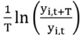refers to the annual growth rate of real per capita GDP in region i from t to t + T; ln(y_i,t) refers to the natural logarithm of real per capita GDP of region i at period t; α is the constant term; β is the convergence coefficient; and ε_i,t is the random error term. If we add controlling variance (innovation capacity in this chapter) in the absolute β convergence model, it will change to Conditional β convergence, as shown in Equation 10.2.

Equation 10.2

In Equation 10.2, P_i,t is the variance reflecting the innovation capacity of region i in year t. Internationally, cross-country regional innovation capacity depends on the potential of producing a series of innovation products, and among them the most important factor is R&D stock (Furman et al. 2002). Chinese scholars have associated regional innovation capacity with the output of innovation results as well as the ability to carry out innovation activities—the most important factor in which is the number of patent applications. In recent years, patents, especially invention patents, have been playing an increasingly noticeable role in China’s regional innovation capacity and economic development and are being taken as an indicator of regional innovation capacity. Provinces and cities with high levels of regional innovation capacity usually have high numbers of invention patents and authorisations. Therefore, in this chapter, the number of invention patent applications is used to measure regional innovation capacity.

We adopt the β convergence test of economic development as noted and measure this using the traditional method in which the spatial effect is not considered. Regions cannot independently develop their own economy; it is instead typically a process closely linked with and affected by the economies of neighbouring regions and those further afield. Spatial effects include spatial dependence and spatial variability: the former refers to the observed value of a sample region being associated with that of other regions; the latter refers to the inhomogeneity of the spatial effect at the regional level due to the heterogeneity of spatial units (Anselin 1988). These two spatial effects correspond to two spatial measurement models: the spatial lag model (SLM) and the spatial error model (SEM). Correspondingly, the SEMs of a regional economy’s absolute β convergence and conditional β convergence are shown in Equations 10.3 and 10.4.

Equation 10.3

Equation 10.4

In Equations 10.3 and 10.4, ρ is the spatial lag coefficient that measures the degree of spatial interaction between observed values of the weight matrix and W is the spatial weight coefficient matrix. The spatial weight matrix is the key to the spatial metering model. At present, most research adopts a simple neighbourhood matrix. However, economic linkages between adjacent regions are not identical and, generally, the degree of interregional interaction is weakened by distance. Given spatial distance is generally inversely proportional to the degree of spatial correlation, this chapter takes the reciprocal of the straight-line distance between the centroids of different regions as the value of the elements in W.

Similarly, the formulas for the SEMs of a regional economy’s absolute β convergence and conditional β convergence are Equations 10.5 and 10.6.

Equation 10.5

Equation 10.6

In Equations 10.5 and 10.6, λ is the spatial error coefficient, reflecting the parameters of the spatial correlation between regression residuals, μ_i,t~N(0,σ²I).

In Equation 10.6, if the estimated value of β is significantly negative, the per capita GDP growth rate of a region is negatively correlated with the per capita GDP level at the initial stage. If the per capita GDP growth rate in economically backward regions is higher than that in developed provinces, there is β convergence of the regional economy. The spatial econometric model is no longer suitable for OLS estimation and, generally, the maximum likehood (ML) method is used to estimate the value of the credible parameter. In addition, according to the estimated value of β, the convergence speed, θ, of a region’s per capita GDP can be calculated and the semi–life cycle, τ, for convergence can be used to show the time it will take economically backward regions to catch up with economically developed regions (Equations 10.7 and 10.8).

Equation 10.7

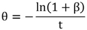
Equation 10.8

Before using the spatial metering model, it is necessary to first determine whether the spatial correlation exists between regional economies, which is usually verified by Moran’s I, first proposed by Moran (1950). The expression is Equation 10.9.

Equation 10.9

In Equation 10.9 is the observed value of region i; n is the number of regions; and ω_ij is the spatial weight value of region i and region j. If the absolute value of Moran’s I is close to 1, it indicates that the spatial correlation of regional innovation capacity is stronger. For the selection of spatial lag and SEMs, Anselin et al. (1997) proposed the following criteria: if LMLAG (Lagrange Multiplier Lag) is statistically more significant than LMERR (Lagrange Multiplier Error) in the spatial econometric model, the SLM is selected; if LMERR is more significant than LMLAG statistically, the SEM is chosen.

The scope of this study is 31 provinces in China (excluding Hong Kong, Macau and Taiwan) and the period studied is 2001–15. All data come from the China Statistics Yearbook for the corresponding year (NBS various years) and the per capita GDP is the price in 2000.

Estimation results and analysis

Regional per capita GDP spatial correlation test

Moran’s I index can be obtained through calculation according to China’s provincial per capita GDP in 2001–15 (see Figure 10.1). Moran’s I indices for regional per capita GDP in 2001–15 all pass the significance test below the level of 5 per cent. Although there is fluctuation in Moran’s I index, all are above 0.3. This indicates that China’s regional economic activities are not in a random state, but, rather, demonstrate the phenomenon of clustering in geographical space; and, in our period, this agglomeration demonstrates, first, a rising trend, but, later, a diminishing trend. In other words, China’s per capita GDP has a strong spatial correlation and provinces with a relatively higher level of economic development are adjacent to each other while economically backward provinces tend to be adjacent to each other.

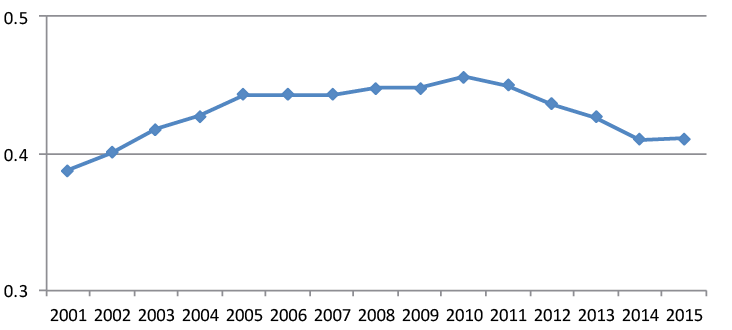
Figure 10.1 Moran’s I index of China’s regional per capita GDP, 2001–15

Source: National Bureau of Statistics of China (various years).

Model and weight selection

For the sake of comparison, this chapter first adopts OLS estimations without considering the spatial effect in the test equation of a regional economy’s absolute β convergence, and the results are shown in Table 10.1.

Table 10.1 Regional economies’ absolute β convergence test results (not considering the spatial effect)

Variances	Estimated value	Standard errors
α	4.2753*	0.5316
β	–0.3307*	0.0593
R2	0.4567
R2 after adjustment	0.5011
Akai information criterion	–18.762

^* significant below 5 per cent

Source: Authors’ estimations.

From Table 10.1, we can see that the convergence coefficient is negative, which is consistent with the expectation and is significant at the 1 per cent level. The model’s fitting coefficient is relatively low, however, indicating that there are problems with the model setting or estimation model. The spatial correlation results of the model fitting residuals show that there is significant spatial autocorrelation of the residual term, the spatial correction coefficient is 0.0281 and the p value is 0.0274. This further shows that the OLS model ignores the spatial correlation between regions, which leads to the error in results. The way to address these issues with the OLS model is to use a spatial weight matrix.

In the selection of spatial weight, we first use the simple neighbourhood matrix used in most studies to correct the OLS model. The spatial model of regional economies’ absolute β convergence is estimated by using the spatial dependence extension package in R language. The results are shown in Table 10.2.

Table 10.2 Regional economies’ absolute β convergence test results (adjacent matrix weight)

Variances	Spatial lag model’s estimated value	Spatial error model’s estimated value
α	3.7585*	0.7463*
β	–0.3028*	0.0637*
ρ/λ	0.0402	0.0189
Log likelihood	12.5247	12.8536
Akai information criterion	–16.891	–16.763

^* significant below 5 per cent

Source: Authors’ estimations.

It can be seen from Table 10.2 that the spatial lag coefficient, ρ, and the spatial error coefficient, λ, are not significant when the adjacency matrix is used as the weight matrix of the regional economic convergence space measurement model. This indicates that the economic development of neighbouring provinces has no statistical significance for a province’s own economic development and the spatial autocorrelation of the error term is not strong, so it has little influence on the model. At the same time, using the Akai information criterion, the SLM and the SEM are –16.891 and –16.763, respectively, which is greater than –18.762 of the OLS model that excludes the spatial effect. If the neighbouring province matrix is used for regional economic convergence, the weight matrix of the model reduces its degree of fit. Adjacent matrices assume that the geographical proximity in the corresponding value in the weight matrix is 1; otherwise, the corresponding value is 0, meaning that the relationship between all adjacent areas is simply regarded as the same without affecting all the non-adjacent regions. In fact, the economic interrelationships between adjacent regions cannot be identical and need to be distinguished; there is still an economic interrelationship in non-adjacent areas.

Absolute convergence test of β regional economy

It can be seen from the above test that, since 2001, the spatial correlation of the economic development level of Chinese provinces is becoming stronger. If spatial correlation between regions is ignored, the reliability of estimated results will be affected. If the neighbourhood matrix is adopted as the weight matrix for the regional economic convergence spatial measurement model, the model cannot be improved. In view of this, in this chapter, the reciprocal of the straight-line distance between different regions is used as the weight of the spatial econometric model.

Since the convergence of regional economic development is often staggered over time (Chen and Guoping 2006), in addition to examining the economic convergence of the entire period, this chapter also divides the period into two (2001–10 and 2011–15) to examine the economic convergence in different periods. To select the appropriate spatial measurement model, this chapter uses the Lagrange multipliers to test the applicability of the SLM and the SEM. The results show that LMLAG is statistically more significant across the entire examination period and also in each of the separate periods, and hence the SLM is selected. The reciprocal matrix of spatial distance is used as the weight to estimate the SLM of absolute b convergence for regional economies, and the results are shown in Table 10.3.

Table 10.3 Results of absolute β convergence of regional economies (reciprocal weight of spatial distance)

Variances	2001–15	2001–10	2011–15
α	5.6449*	3.9415*	1.0277*
β	–0.3706*	–0.2143	–0.0898*
ρ	0.7688**	1.1202**	0.5223**
Log likelihood	12.2190	14.5290	35.6480
Akai information criterion	–16.438	–21.058	–63.296

^* significant below 5 per cent

^** significant below 1 per cent

Source: Authors’ estimations.

The Akai information criterion of the SLM is smaller than that of the OLS model without considering the spatial effect. This shows that if the reciprocal of spatial distance is used as the weight matrix of regional economic convergence, the degree of fit for the weight matrix of the model can be improved. The increase in the logarithmic likelihood also shows that the model is superior to the regional economic convergence spatial model with the adjacent matrix as the weight matrix. The results also show that the spatial lag coefficient, ρ, is 0.7688 and the significance test at the 5 per cent level shows that there is significant positive spatial autocorrelation in interprovincial economic development in China. That is, there is an interprovincial spillover effect on economic development: a region’s economic development can promote the economic development of adjacent regions. The convergence coefficient, β, is –0.3706, which is significant at the 1 per cent level. This shows that the speed of economic development in each province is negatively correlated with its initial economic level. In other words, the provinces with relatively high levels of development will slow their growth rate in the beginning, while the provinces with relatively low economic levels will have a higher economic growth rate.

In sum, the results suggest that regional economic development in China shows a general convergence trend from 2001 to 2015. In terms of the results of the economic convergence test for 2001–10, the convergence coefficient, β, is not statistically significant, indicating that there is no convergence phenomenon in China’s regional economic development during this period. However, regional economic development is convergent in 2011–15: the convergence coefficient, β, is –0.0898, which is significant at the 1 per cent level.

In fact, in terms of the Gini coefficient, the Tyler index, the variation coefficient, the Herfindahl index and other indices that measure the gap in regional economic development, there is also a declining trend during the period under examination, as shown in Figure 10.2.

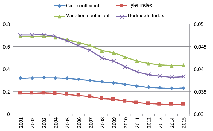
Figure 10.2 Four indicators of the gap in regional economic development

Note: Indicators are calculated using the R language ineq extension package, and the Herfindahl index is on the secondary axis.

Source: National Bureau of Statistics of China (various years).

It can be seen from Figure 10.2 that although the Gini coefficient, the Tyler index, the variation coefficient and the Herfindahl index fell as a whole from 2001 to 2015, they remained relatively stable over the period 2001–06, and thereafter demonstrated a declining trend. This validates the empiriral results of this chapter from one side. In addition, according to the estimated value of β, it is also possible to calculate that the convergence rate of per capita GDP in China from 2001 to 2015 was 3.307 per cent and the half–life cycle of convergence was 20.95 years, which means it will take 20.95 years for economically backward regions to catch up with economically developed regions.

The influence of regional innovation capacity on economic convergence

In addition to absolute convergence analysis, this chapter introduces regional innovation ability to the spatial model and analyses its influence on economic convergence. The estimated results of the SLM of the β convergence test of regional economic conditions are shown in Table 10.4.

Table 10.4 Results of the β convergence test of regional economic conditions

Variances	2001–15	2001–10	2011–15
α	4.4207*	2.7380*	1.4669*
β	–0.3449*	–0.1969	–0.1356*
£	0.0059**	0.0105	0.0401
ρ	1.3102**	0.6321	0.4528
Log likelihood	13.0045	13.7573	36.2550
Akai information criterion	–16.009	–17.515	–62.510

^* significant below 5 per cent

^** significant below 1 per cent

Source: Authors’ estimations.

The results of the β convergence test of regional economic conditions in 2001–15 show that the spatial lag coefficient, ρ, is 1.3102 and passes the significance test at the 5 per cent level. The spatial lag coefficient of the β convergence of regional economic conditions is larger than absolute β convergence, indicating that the spread of China’s innovation activities and innovation results helps improve the interaction of provincial economic development. The conditional convergence coefficient, β, was –0.3449 between 2001 and 2015, and significant at the 1 per cent level, suggesting that China’s economic development level has conditional β convergence in the whole economic space. The regression coefficient, £, was 0.0059 and significant at the 5 per cent level, indicating that the economic growth rate increase of 5.9 percentage points is associated with a 1 per cent increase in innovation capacity. From 2001 to 2010, the convergence coefficient, β, was statistically insignificant, indicating there was no convergence phenomenon in China’s regional economic development, even if the control factor was added, in this period. However, regional economic development in 2011–15 achieved conditional convergence; the convergence coefficient, β, was –0.1356, which was significant at the 1 per cent level. This shows that, in recent years, China’s radiation and leading effects of regional innovation have gradually appeared, which have promoted the convergence of regional economic development.

Similarly, according to the estimated value of the conditional convergence coefficient, β, it can be calculated that, after innovation capacity is taken into account, the conditional convergence speed of regional per capita GDP is 3.021 per cent, which is 0.6 per cent slower than the speed of absolute convergence; and, in turn, the half–life cycle of the conditional convergence is 22.94 years. In other words, after the influence of regional innovation capacity is taken into account (and this is slower in economically backward regions), this innovation lag alone will add 3.87 years to the time needed to catch up with economically developed regions, compared with the result when regional innovation capacity is not considered.

Results, conclusion and policy recommendations

In this chapter, the inverse distance between different regions is used as the weight matrix to analyse the actual per capita GDP of 31 provinces and municipal equivalents in China from 2001 to 2015, and the influence of regional innovation ability on economic convergence is discussed. The results show that: 1) after considering the spatial effect, China’s regional economic development has both conditional convergence and absolute convergence; 2) in recent years, the trend in China’s regional economic development convergence is more obvious than before; and 3) after regional innovation capacity is taken into account, the speed of convergence of China’s regional economy deteriorates.

There is absolute convergence in China’s regional economic growth, and this conclusion cannot be drawn from the OLS framework. Although from the perspective of economic development, absolute convergence is not obvious in the short term, in the long term, there is a trend of absolute convergence in China, and this trend is becoming increasingly obvious. Therefore, China’s regional economic convergence is consistent with the original prediction of the neoclassical growth model, rather than the result achieved after controlling the influence of relevant variables. This also shows that it is not feasible nor would it be effective for China to adopt the growth poles theory to develop its economy. Although geographical conditions, resource endowment and other factors may have a negative impact on the convergence trend, with the gradual establishment and improvement of the market economy, there is still obvious potential for convergence in China’s regional economic growth.

China is undergoing economic transformation, so how to control and narrow the regional development gap through effective intervention is not only one of the key objectives of China’s current macroeconomic regulation, but also an important problem that needs to be solved urgently. Romer (1990) and many other researchers suggest that the level of human capital is an important factor affecting the rate of economic convergence. The research in this chapter shows that innovation ability also has a significant impact on the speed of economic convergence. If the spatial pattern of the excessive concentration of innovation resources and the serious imbalance in innovation capacity cannot be improved, China’s economic development will step into the stage of widening regional disparity caused by innovation. Therefore, in formulating innovation policy, the Chinese Government should pay attention to the spatial interaction mechanism and make full use of the regional innovation resource endowment and differences in innovation ability to reduce the gap in regional economic development.

References

Anselin, L. (1988), Spatial Econometrics: Methods and models, Dordrecht: Kluwer Academic Publishers. doi.org/10.1007/978-94-015-7799-1.

Anselin, L., Varga, A. and Acs, Z. (1997), Local geographic spillovers between university research and high technology innovations, Journal of Urban Economics (42): 422–48. doi.org/10.1006/juec.1997.2032.

Barro, R. J. and Sala-i-Martin, X. (1992), Convergence, Journal of Political Economy 100(2): 223–51. doi.org/10.1086/261816.

Baumol, W. J. (1986), Productivity growth, convergence, and welfare: What the long-run data show, American Economic Review 76(5): 1072–85.

Cai, F. and Yang, D. (2000), The convergence and difference of economic growth in China: The Enlightenment to the Western development strategy, Economic Research (10): 30–7.

Carrington, A. (2003), A divided Europe? Regional convergence and neighbourhood spillover effects, Kyklos 56(3): 381–93. doi.org/10.1046/j.0023-5962.2003.00226.x.

Chen, X. and Guoping, L. (2006), Analysis of spatial panel data model of regional economic convergence in China, Economic Science (5): 5–17.

Furman, J. L., Porter, M. E. and Stem, S. (2002), The determinants of national innovative capacity, Research Policy 31(6): 899–933. doi.org/10.1016/S0048-7333(01)00152-4.

Lin, G., Zhihe, L. and Mei, W. (2005), An empirical study on the spatial measurement of regional economic convergence in China: 1978–2002, Economics Quarterly (B10): 67–82.

Lin, Y. and Lui, M. (2003), China’s economic growth convergence and income distribution, World Economy (8): 3–14.

Moran, P. A. P. (1950), Notes on continuous stochastic phenomena, Biometrika 37(1): 17–23. doi.org/10.1093/biomet/37.1-2.17.

National Bureau of Statistics of China (NBS) (various years), China Statistics Yearbook, Beijing: China Statistics Press.

Pan, W. (2010), Regional economic disparity and convergence in China, Chinese Social Sciences (1): 72–84.

Perroux, F. (1950), Economic space: Theory and applications, Quarterly Journal of Economics 64(1): 89–104.

Ren, L., Xue, J., Liu, Y-g. and Wang, Z. (2014), Research of R&D marginal productivity driving regional economic convergence, Studies in Science of Science (11): 1661–7.

Romer, P. M. (1990), Endogenous technological change, Journal of Political Economy 98(5): 71–102. doi.org/10.1086/261725.

Romer, P. M. (1994), The origins of endogenous growth, Journal of Economic Perspectives (5): 3–22. doi.org/10.1257/jep.8.1.3.

Shen, K. and Jun, M.(2002), A study on the characteristics of ‘club convergence’ in China’s economic growth and its causes, Economic Research (1): 33–9.

Solow, R. M. (1956), A contribution to the theory of economic growth, Quarterly Journal of Economics 70(1): 65–94. doi.org/10.2307/1884513.

Wang, Z. and Zhaopan, G. (2002), The multiple equilibrium and the precursors of China’s regional economic development, Chinese Social Sciences (4): 31–9.

Wei, H. (1997), China’s regional economic growth and its convergence, China Industrial Economy (3): 31–7.

Wu, Y. (2006), Spatial econometric analysis of regional economic growth convergence in China, Quantitative Economic, Technical and Economic Research (12): 101–8.

Wu, Y. (2007), Research on Spatial Econometrics of Regional R&D, Knowledge Spillover and Innovation in China, Beijing: People’s Publishing House.