21. Rural-to-urban migration and migrants’ labour market performance, 2008–16

Bob Gregory and Xin Meng

In 1978, the Chinese economy was segregated into two parts: the rural and the urban economies. Migration was forbidden. At that time, about 80 per cent of the population lived and worked in the rural sector. Economic reforms initiated in the agricultural sector in 1978 produced significant productivity increases and released a large portion of the rural workforce to move into the more productive nonagricultural sector to work. However, throughout the 1980s, rural-to-urban migration was still largely prohibited. Workers released from the agricultural sector, combined with the agricultural surplus and migration restrictions, created the conditions for the development of township and village enterprises (TVEs), which absorbed surplus labour and played a major role in generating growth during this period.

It was not until the early 1990s, when the open-door policy brought large-scale foreign direct investment (FDI) into Chinese cities and the demand for unskilled workers increased in locations away from the village, that the government gradually loosened rural–urban migration restrictions. This movement of migrant labour generated rapid economic growth associated with construction in cities and double-digit export growth. During this period, rural–urban migration increased, from 25 million in 1990 to 170 million in 2016 (see Figure 21.1). It is difficult to imagine how China could have grown so quickly for so long without this massive reallocation of labour.

Although labour could move to seek employment, there were still substantial restrictions in place to prevent permanent migration. As a result, most migration was temporary and many workers moved back and forth between villages and cities depending on their personal circumstances. There has been some weakening of these ‘permanent’ migration restrictions, but such reforms have been slight and longer city stays, which are increasingly occurring, are still largely confined to migrants with temporary status.

It now seems that the old growth model that has served China so well—built on increasing temporary migration to large cities—has come to an end. In the future, the relationship between rural–urban migration and economic growth will be very different, as the drivers of economic growth shift from manufacturing exports and construction in large cities to more diversified activities, primarily located in small cities. Large numbers of workers will continue to leave agricultural production, seeking higher incomes, but their employment destinations will change as they move to jobs much closer to home.

To a significant degree, the fundamental change in migration flows has already begun. Between 1998 and 2007, 100 million migrants augmented the large-city workforce. Between 2007 and 2016, the migrant addition was 20 million, but, between 2014 and 2017, there was almost no increase in migrant numbers in large cities.

The large shift in migration flows away from large cities towards small cities and rural towns has important implications for economic growth, economic policy and the balance of markets and government regulation as determinants of what happens to future large-scale labour reallocations. It is important therefore, as part of understanding this ongoing transition from one growth model to another, to map out and understand the nature of the migrant flows to the large cities and how economic outcomes in cities and villages have responded as the migration flows have changed. To begin to do this, we use data from the Rural–Urban Migration in China (RUMiC) survey that began collecting data in large cities and villages from 2008, just before the migration inflows to the large cities began to substantially moderate. The RUMiC survey extends to 2016, by which time significant net migration inflows to large cities had ceased.

The data reveal, to a large extent, what might be expected when migration inflows slow. We see, for example, substantial ageing of the migrant stock as the relative importance of young migrant inflows declines. Other migrant outcomes are also changing in expected ways, but only slowly, while others, to this point, seem little affected.

But one outcome of special interest to economists is not changing as expected. Large migrant inflows were encouraged by relaxation of government migration restrictions and the large wage gaps between the migrant wage in the city and what the migrant could earn at home. It might be expected therefore that large migrant inflows, increasing labour supply in the cities and reducing labour supply in hometowns, would gradually erode this income gap. As the gap narrows, net migration would be expected to slow as labour reallocation in China moved to a new equilibrium growth path. But this story does not seem to be fully consistent with the facts. As expected, the earnings gaps between the migrants’ receiving cities and their hometowns are large at the beginning of the period, when migrant inflows are large, but what is not expected is that the income gaps are much the same at the end of the period, when there are very small additional net migration inflows. The migration flows seem to have stopped, but there is little evidence in our data of any obvious equalisation of relative labour market outcomes in the migration-sending rural hometowns and the migrant-receiving cities. So there are two puzzles here. First, why were the rapid and large migrant inflows ineffective in reducing the relative rewards for migration? Second, why has the net migration flow stopped when the relative rewards for migration are much the same as they were during the high migration period? These are important questions that we cannot fully answer here, but we make a start.

Consideration of these questions suggests that migration flows in China depend on the individual decisions of workers to move and government policies surrounding those decisions. The government has always played a large role in determining the geographic allocation of labour and it seems clear government policy has now changed. The new policy is directing immigrants away from large cities and towards small, more remote cities.

The economic implications of this new policy, and its interactions with decisions about where and whether to migrate, are particularly interesting. The old policy can be thought of as the government responding to economic forces pulling workers to cities and to excess rural labour; however, the new policies do not seem to be a response to the usual economic forces. The wage gap between cities and rural villages remains and hence the economic return to moving migrants to cities, at least measured by this metric, remains. It is not as though the absorption capacity of large cities, as measured by relative wages, has changed in any significant way. Hence, it appears the new policy is forgoing the economic gains that would come about by narrowing the wage gap between large cities and rural towns in pursuit of some other objective.

Given the availability of Chinese data, it is not a straightforward matter to disentangle the role of government policy on one hand and economic incentives on the other as determinants of the large changes in migrant flows. Hence we are forced to take a very indirect approach and this chapter is mainly descriptive, documenting what have been important migrant outcomes in large cities, what has changed and what has not. We see this as the laying of a firmer foundation on which to build an assessment of past migration impacts and to support various conjectures of what is likely to happen in the future. To some extent, the description updates the chapter by Meng (2013) for the 2013 China Update, but this chapter directs more attention to changing patterns of outcomes and how they might relate to changing migration flows.

The next section provides a general picture of the changing migrant flows. Section two examines the characteristics of the migrant stock in large cities. Section three documents the economic performance of migrants, while section four analyses the changing determinants of migrant earnings. Section five considers the changing pattern of migrants’ wages across cities and conclusions are given in section six.

The changing flows of rural-to-urban migration

In Chinese statistics, there are two different definitions of rural-to-urban migrants (in Chinese, Nong Min Gong—literally, ‘farmers turned workers’). The first definition refers to anyone with ‘rural household registration’ (hukou) who is not working in agriculture, including those who are working in a nonfarming job in their rural hometown. The second definition refers to those who become nonfarm workers by moving to cities—in other words, ‘rural-to-urban migrants’. In recent years, the National Bureau of Statistics (NBS) has published the numbers for both definitions (see Figure 21.1).

In 1990, due to government restrictions, fewer than 25 million rural workers moved to the city to work, while a larger number worked at rural TVEs in their hometown. By the late 1990s, as China’s ‘open door’ policy attracted more and more FDI, the demand in the cities for unskilled labour increased. As a result, rural-to-urban migration accelerated. The fastest period of migration growth was after China joined the World Trade Organization (WTO) and until the Global Financial Crisis (GFC). Immediately after the GFC, due to the reduction in global demand for Chinese exports, the increase in migration rates dropped sharply. Net migration appears to have increased little over the past three years. The demand for Chinese exports has not bounced back to pre-GFC levels and China’s economic growth strategy has changed from export-driven to domestic demand–driven growth. As a result, most nonfarm job growth for rural hukou workers involves those who stay at home and work in nearby small towns.

To what extent the slowdown in migration to large cities is a response to market forces and to what extent it is the result of government policy is unclear. Our description of migrant outcomes will help us address this question. At this point, the data we examine suggest that policy shifts are the key determinants of the changing long-run pattern of migration flows and we note that the ‘National New Urbanisation Plan 2014–2020’ reinforces this judgement. The plan suggests the government had not let go of the fear of large or mega-city development and has become more determined to direct migrants towards small cities and to ignore the agglomeration advantages of further large-city development (see Meng 2014).¹ Despite economists’ advocacy of the advantages to be gained from large or mega-city agglomeration effects in the economic development process, further migration to big cities seems to be a lost cause for now.

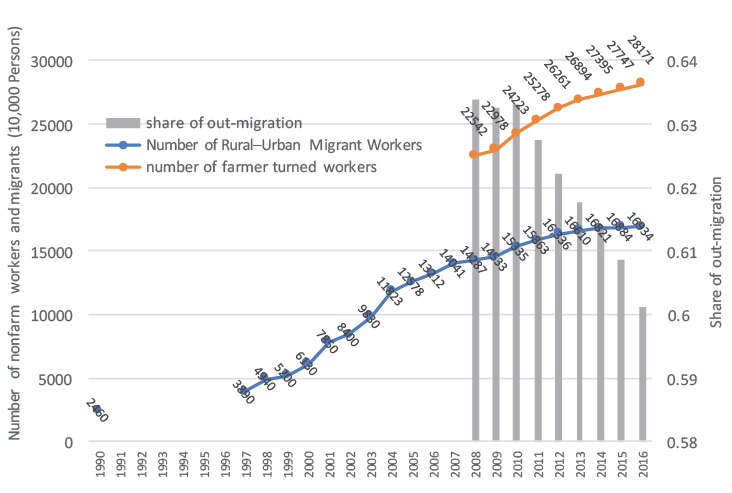
Figure 21.1 China’s ‘rural’ workforce working in nonfarm jobs

Sources: The rural–urban migration data for 1990 are the authors’ own calculation, using 1990 population census data; 1997 data are from World Bank (2009: Fig 2.41); data for 1998–2008 are from NBS (various years [b]) and thereafter from NBS (various years [a]).

The redirection of migrant inflows are impacted by policies at all levels of government. Local city restrictions on migrant access to social services and social insurance are one factor discouraging migration inflows to big cities, while large-scale central government investment in rural and small towns is a factor encouraging migration inflows to small cities. In many instances, such policies have an impact not only on migration inflows, but also directly on migrants who are already in large or mega-cities. In December 2017, for example, the Beijing city government heavy-handedly implemented a 40-day clean-up campaign to rid the city of unsafe buildings, in which about 8.2 million migrant workers had lived for decades. Many of these migrants subsequently left Beijing.

Characteristics of migrant workers

The RUMiC survey combines a longitudinal sample (panel old households) and a repeated cross-section sample (representative new households). The survey is randomly refreshed from each of the 15 cities in each survey year. Using these data, we present basic statistics to show the characteristics of the migrants and whether these have changed.

Table 21.1 Summary statistics of individual migrant characteristics

					Ever married		Opinion/attitude
Year	Age	Male	Married	Years of schooling	Divorced/remarried	No. of children	Stay in city perm-anently	Happy
	[1]	[2]	[3]	[4]	[5]	[6]	[7]	[8]
2008	31.02	0.61	0.62	9.11	0.029	1.33	0.60	0.89
2009	32.04	0.59	0.65	9.17	0.032	1.36	0.64	0.89
2010	32.34	0.59	0.64	9.28	0.028	1.39	0.62	n.a.
2011	33.01	0.56	0.68	9.23	0.034	1.40	0.62	0.89
2012	34.17	0.56	0.73	9.21	0.030	1.44	0.64	0.92
2013	35.20	0.55	0.75	9.21	0.036	1.48	0.67	0.93
2014	36.05	0.55	0.77	9.15	0.039	1.49	0.70	0.93
2015	36.36	0.55	0.77	9.23	0.040	1.52	0.64	0.93
2016	36.82	0.55	0.77	9.32	0.041	1.52	0.69	0.92
Panel (old households)
2008	31.02	0.61	0.62	9.11	0.029	1.33	0.60	0.89
2009	33.08	0.58	0.73	9.01	0.036	1.39	0.69	0.88
2010	33.56	0.58	0.73	9.23	0.025	1.37	0.68	n.a.
2011	33.93	0.56	0.75	9.31	0.031	1.41	0.66	0.90
2012	34.95	0.56	0.76	9.19	0.032	1.44	0.69	0.93
2013	35.95	0.55	0.79	9.19	0.039	1.47	0.71	0.93
2014	36.59	0.55	0.80	9.23	0.037	1.51	0.71	0.93
2015	37.49	0.55	0.81	9.20	0.042	1.51	0.67	0.92
2016	37.78	0.55	0.81	9.28	0.041	1.52	0.71	0.93
Representative (new households)
2008	31.02	0.61	0.62	9.11	0.029	1.33	0.60	0.89
2009	31.43	0.59	0.60	9.27	0.029	1.41	0.61	0.89
2010	31.12	0.60	0.55	9.32	0.033	1.34	0.56	n.a.
2011	31.62	0.56	0.59	9.12	0.040	1.43	0.55	0.87
2012	32.58	0.57	0.66	9.26	0.025	1.44	0.54	0.90
2013	33.53	0.56	0.66	9.25	0.029	1.45	0.60	0.94
2014	34.89	0.56	0.71	8.99	0.044	1.54	0.68	0.93
2015	33.98	0.54	0.69	9.31	0.036	1.48	0.58	0.93
2016	34.39	0.56	0.67	9.41	0.042	1.52	0.63	0.91

n.a. = not available

Table 21.1 presents the mean values of a selection of characteristics for those aged 15–64 years from each of our samples. Based on the representative sample, the average age of a migrant worker in our large cities has increased by three years over the nine years of data collection (from 31 to 34 years of age), there has been a slight increase in the number of women joining the migrant workforce (from 39 per cent to 45 per cent), more migrant workers are married (from 62 per cent to 68 per cent) and migrants’ years of schooling have increased slightly (by 0.3 years). In addition, among ever-married migrants, the divorce rate (including those who have remarried) has increased (from 2.9 per cent to 4.2 per cent) and the number of children has increased, too (by 0.2 per family). These changes—particularly the increase in migrants’ age, the marriage rate and the number of children—are to be expected when migration inflows substantially reduce. But they provide no obvious reasons for the fall in migration inflow rates.

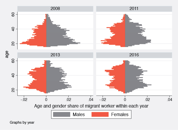
Figure 21.2 Age distribution of migrant workforce (full sample)

Source: Authors’ own calculation from RUMiC data.

Averages often disguise important changes, so it may be worthwhile to look at changes in the distribution of some of these variables. Figure 21.2 indicates substantial changes in the migrant age distribution. In 2008, the dominant proportion of the migrant workforce was in the 16–35 year age group (65 per cent of men and 70 per cent of women). By 2016, the workforce was divided almost equally between those below 35 years of age and those above. The number of those above 35 years of age increased from 35 per cent for men and 30 per cent for women in 2008 to 40 per cent and 48 per cent, respectively, in 2016 based on a representative sample. The increase was largest for older women.

The question that naturally arises is whether the increase in older workers is the result of new older migrant inflows or a natural outcome of migrants staying longer in the cities. Changes in migrants’ current job tenure may throw some light on this issue. If most of the older group comes from new inflows, we would expect their current job tenure to be relatively short.

Figure 21.3 shows that men and women over 35 years of age have been in their current job for quite a long time and the proportions of those in the long tenure categories have been increasing in recent years. In 2008, 40 per cent of women and 52 per cent of men aged over 35 years had five or more years of tenure in their current job. By 2016, the ratios had increased to 70 per cent for women and 72 per cent for men, suggesting a substantial part of the growth in the older age groups is being generated by migrants ageing in the city rather than by new inflows. These results are perhaps to be expected as the aggregate net migrant inflows have dropped dramatically.

Total Sample	Representative Sample

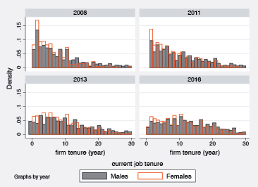
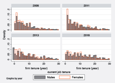
Figure 21.3 Current job tenure for workers aged 40 and above

Source: Authors’ own calculation from RUMiC data.

The mean years of education have increased by 0.3 of a year. What can be said about the source of this increase? Figure 21.4 indicates that the marginal improvement in average education levels is generated mainly by a lift in the proportion of workers with a three-year college qualification, at the expense of junior and senior high school graduates. This is true for both men and women. A more striking observation from Figure 21.4, however, is that the proportion of women who are illiterate or have only primary school education has increased over time, from 16 per cent to 23 per cent, while the same pattern is not observed among men.

Total Sample	Representative Sample

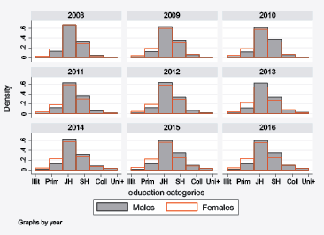
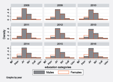
Figure 21.4 Education distribution by gender

Key: Illit = illiterate; Prim = primary school; JH = junior high school; SH = senior high school; Coll = three-year college; Uni+ = university.

Source: Authors’ own calculation from RUMiC data.

Does this pattern suggest that the education level for rural women coming to the city has worsened or does it simply reflect the changing demographic structure of the current migrant female labour force—that is, a larger proportion of older women are now in the migrant workforce than before? To answer this question, we divide our sample into five different birth cohorts (1946–59, 1960–69, 1970–79, 1980–89 and 1990–99) to see whether those who were born in the 1980s and 1990s have a similar education distribution as those who were born earlier. If the young cohorts are better educated, the observed increase in the poorer educated must be due to the increase in the proportion of the older workforce in recent years. Figure 21.5 shows that women’s educational attainment improved significantly in the recent birth cohorts. Thus, the older women who have remained in the city workforce have generated the increase in the proportion of poorer educated female workers.

Total Sample	Representative Sample

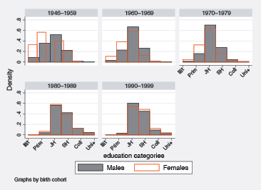
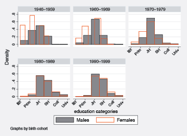
Figure 21.5 Education distribution by birth cohort and gender

Key: Illit = illiterate; Prim = primary school; JH = junior high school; SH = senior high school; Coll = three-year college; Uni+ = university.

Source: Authors’ own calculation from RUMiC data.

To this point the changes in means and distributions of demographic variables seem slight, much as might be expected, and do not appear to provide any obvious answers for why net migration inflows have fallen so much.

The RUMiC survey also asks respondents a range of attitudinal questions, which might get more directly to the reasons for the slowdown of migration inflows. One question asked is: ‘If policy allows, how long do you want to stay in the city?’ The answers are particularly important. The majority of the sample, between 60 per cent and 70 per cent, wishes to stay in the city permanently, and this proportion has increased marginally over the data period (Column 7 of Table 21.1). Among migrants in cities there seems to be no attitudinal change that might explain why migration inflows have fallen. Indeed, preference for staying in the city is increasing.

RUMiC also asks migrants: ‘Considering all aspects of your life, are you (1) very happy, (2) happy, (3) not very happy, or (4) very unhappy?’ Table 21.1 presents the proportion who answer ‘very happy’ or ‘happy’. More than 90 per cent of migrants fall into this category and, again, there has been no significant change that might explain the fall in migration inflows.²

The means of the data presented in Table 21.1, and their distributions, support two judgements: 1) demographic outcomes move in the expected direction when net migration inflows slow dramatically, and provide no obvious clues for why net migration inflows have fallen; and 2) attitudinal data also provide no significant evidence of increased dissatisfaction with city life.

Perhaps explanations for reduced migrant inflows can be found in the more direct measures of labour market outcomes, which may reflect large falls in the demand for migrant labour in large cities?

Migrants’ labour market performance

Many migrants are drawn to cities by the large earnings gap between rural and urban areas. How has this gap changed over time and how does it relate to changing migration flows?

The RUMiC survey asked each worker: ‘If you did not migrate, how much would you have earned per month at your rural hometown?’ Based on these data, together with the migrants’ reported monthly earnings in the city, we calculate the mean wage differential between the hometown and the city.

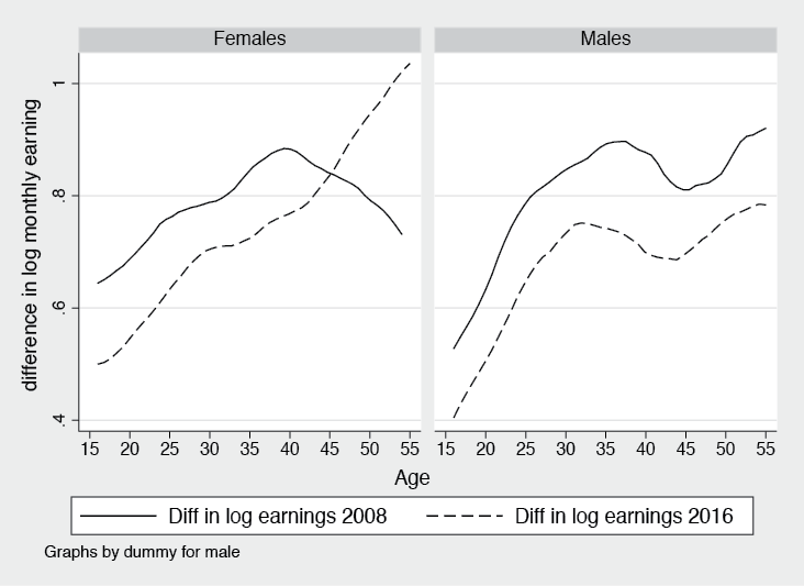
Figure 21.6 Log monthly earnings gap between city and rural hometown

Source: Authors’ own calculation from RUMiC data.

In 2008—the year when net migration inflows were high—the difference in the average wages in the city and the hometown is 86 per cent (including for the self-employed). In 2016, when net migration inflows had ceased, the earning gap had reduced to 71 per cent. If only wage and salary earners are included, the gap in 2008 is 77 per cent and in 2016, 70 per cent. So earnings gaps have fallen, and the direction of change is as might be expected if this change were to reduce migration inflows. But is this fall in the earnings gap sufficient to cause net migration inflows to virtually cease? It seems unlikely and at this point our judgement is that a city premium of 70 per cent is still very high and the fall in the earnings gap seems slight and insufficient to explain such a large change in migration inflows.

Large earnings gaps and small falls through the period when migration inflows have fallen so much are found among all the groups we consider. Figure 21.6 presents the gaps by gender and age group for the first and last years of the survey. The failure of the earnings gap to narrow significantly by age and gender is yet another sign that the current trend for more rural workers to stay in their rural hometowns to work seems not to be a response to individual incentives, as is normally thought in market economies.

Although the earnings gap between the city and the home village seems to have narrowed slightly, real earnings in both the city and the home village have increased very considerably, and it seems probable that real and rapid income growth in the city is likely to validate the decision to migrate.

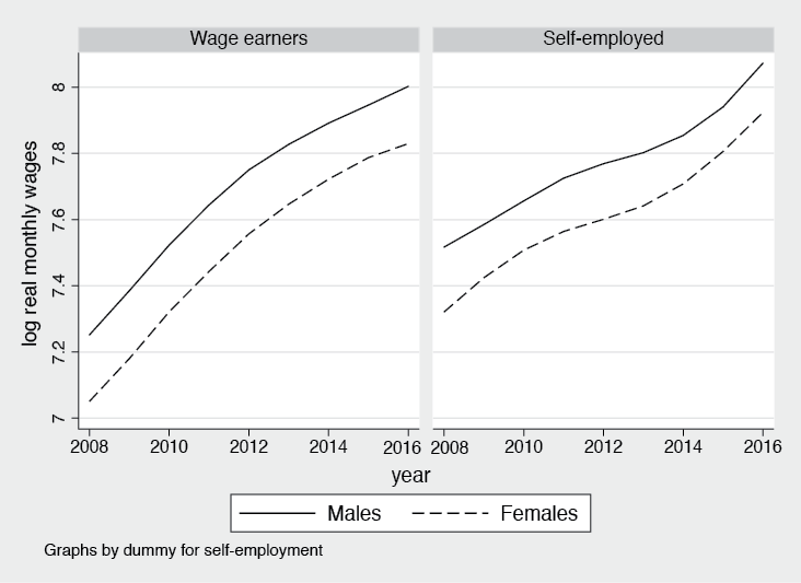
Figure 21.7 Log monthly real wages/income by gender and employment status

Source: Authors’ own calculation from RUMiC data.

The left panel of Figure 21.7 shows that, in the past nine years, migrants’ real wages increased by about 70 per cent for both male and female workers. The period of fastest growth was before 2013; thereafter the speed of increase slowed somewhat. Women have shared equally in this high growth rate, although they earn about 20 per cent less than men. Net income³ for self-employed workers has also grown quickly, but not as fast as that for the wage/salary earners (Figure 21.7, right panel). Their net income increased by about 40 per cent over the nine years. Self-employed women were making about 20 per cent less than men at the beginning of the period, but the gap reduced somewhat at the end of the period, to about 15 per cent.

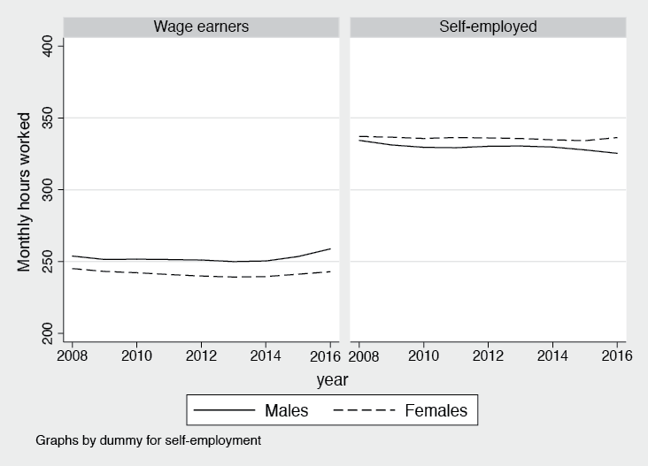
Figure 21.8 Monthly hours worked by employment status

Source: Authors’ own calculation from RUMiC data.

Of course, earnings are not the only thing that matter, but also how much work needs to be done to receive these earnings. There have been limited changes in the long hours worked by wage earners and the self-employed (Figure 21.8). One could imagine an adverse reaction from migrants to these long hours worked and a demand for shorter hours as real incomes increase, but there is little evidence of any widespread dissatisfaction, as indicated by migrants’ willingness to stay in the city permanently and their level of happiness (see the earlier discussion about the results from Table 21.1). Nevertheless, the long hours worked are striking.

If we assume for wage earners that an eight-hour day, six-day week are ‘normal’ then the normal monthly working hours should be no more than 207 hours. Both male and female migrant wage/salary earners report an average of 40 or more hours above this ‘normal’ monthly limit (more than 250 hours monthly), and there has been no noticeable change over our data period.

The self-employed also work very long hours—on average, close to 340 hours a month, or more than 11 hours a day for a seven-day week. How do these long work hours relate to income earned?

For the self-employed, average monthly net income levels have always been above the wage earner average, but their average hourly income has always been lower (Figure 21.9). In recent years, however, the relative position of the self-employed has improved. Between 2013 and 2016, the annual average real hourly earnings growth for wage and salary earners barely reached 1.5 per cent. For the self-employed, however, the growth was 11 per cent.

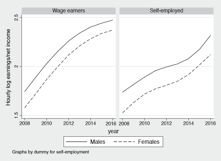
Figure 21.9 Hourly real log earnings/net income, by employment status

Source: Authors’ own calculation from RUMiC data.

The stronger hourly income growth among the self-employed may be one reason their share among migrant workers has been increasing recently. For the representative sample, the proportion of migrant workers who were self-employed in 2008 was 24 per cent; by 2016, the ratio had increased to 29 per cent.

The change in the migration inflows should also impact on the length of stay in the city. Data in Figure 21.10 show that, on average, the number of years since first migrating to the city to work increased by four to five years between 2008 and 2016, and the increases occurred mainly after 2010 (post the GFC).⁴ Self-employed migrant workers, on average, have been in cities for four to five years longer than wage and salary earners, and the increments over the past nine years are about the same as for their wage and salary counterparts. The lengthening of the average time since arrival in the city suggests the dramatic slowdown in net migration to the city has been generated primarily by reduced inflows of new workers rather than an increased exodus of workers who have been in the cities for a long time. This result is consistent with the ageing of the migrant stock.

There is no indication, however, that the slowdown of migrant inflows has impacted on job turnover. Migrant wage/salary earners have been in their current job for three to four years and this has not changed much over the past nine years. The current job duration for the self-employed—an average of six to seven years—is almost double that of the wage/salary earners, but it too has not significantly increased.

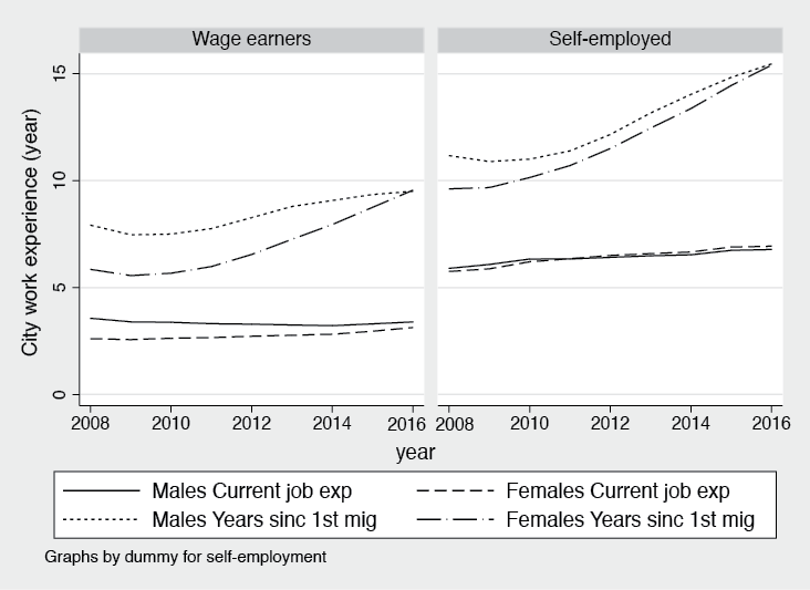
Figure 21.10 Years since first migration and current job experience

Source: Authors’ own calculation from RUMiC data.

We also look at social insurance coverage and whether migrants have written contracts that legalise their employment position and protect their rights in case of disputes. Table 21.2 presents the social insurance coverage for all workers, for wage/salary earners and for self-employed workers, separately. Columns 1–3 present the total number of insurance types held by migrant workers. By law, employers must pay (jointly with employees) into five different insurance funds: health, unemployment, pension, workplace injury and housing. In 2008, the average migrant in the representative sample had 0.6 of the five types of insurance, with wage/salary earners having 0.8, while the self-employed had 0.04. Columns 4–6 and 7–9 list two of the most important insurance types for migrants: health and pension. For all workers, the incidence of these types of insurance has increased from 10 per cent and 17 per cent coverage in 2008, respectively, to 28 per cent for both in 2016. The most impressive improvement was made among wage/salary earners, rising from 13 per cent for health insurance and 21 per cent for pension insurance in 2008, to 39 per cent for both by 2016. These outcomes suggest an improving work environment for migrants. For self-employed workers, however, there is virtually no coverage.

From 2010, the RUMiC survey asked whether migrant wage/salary earners had signed a written contract with their employer. One important aim of 2008’s New Labour Law was to ensure that workers have a written contract so any industrial relations dispute can be resolved through legal channels (Meng 2017). The law clearly states that if a written labour contract has not been signed with an employee within one year, the employer will be deemed to have signed an open-ended contract or will incur a penalty that requires the employer to double the salary paid to the employee (NPC 2007). The results from the RUMiC survey indicate that in 2010 about 49 per cent of wage/salary earners already had a written contract with their employer. The ratio did not change much. By 2016, about 53 per cent were covered by written contracts.

It seems the implementation of the New Labour Law has been more successful in achieving written contracts than in the provision of social insurance; however, over time, not much progress has been made.

Table 21.2 Social insurance coverage

	Number of social insurance funds			Percentage of health insurance coverage			Percentage of pension insurance coverage
All workers	Panel sample	Rep. sample	Total	Panel sample	Rep. sample	Total	Panel sample	Rep. sample	Total
	[1]	[2]	[3]	[4]	[5]	[6]	[7]	[8]	[9]
2008	0.61	0.61	0.61	0.10	0.10	0.10	0.17	0.17	0.17
2009	0.59	0.62	0.61	0.12	0.10	0.11	0.16	0.17	0.17
2010	0.85	0.66	0.75	0.22	0.17	0.20	0.22	0.15	0.18
2011	0.84	0.76	0.81	0.19	0.16	0.17	0.21	0.20	0.21
2012	0.93	1.11	0.99	0.21	0.28	0.23	0.24	0.29	0.25
2013	1.11	1.02	1.08	0.27	0.24	0.26	0.28	0.24	0.26
2014	1.03	0.92	0.99	0.25	0.23	0.24	0.25	0.23	0.25
2015	1.06	1.07	1.06	0.26	0.25	0.25	0.25	0.25	0.25
2016	1.20	1.20	1.20	0.28	0.28	0.28	0.29	0.28	0.29
Wage/salary earners
2008	0.78	0.78	0.78	0.13	0.13	0.13	0.21	0.21	0.21
2009	0.95	0.79	0.84	0.18	0.13	0.15	0.26	0.22	0.23
2010	1.29	0.84	1.05	0.33	0.22	0.27	0.33	0.20	0.26
2011	1.31	0.98	1.17	0.29	0.20	0.25	0.34	0.26	0.30
2012	1.50	1.45	1.48	0.34	0.36	0.35	0.38	0.37	0.38
2013	1.86	1.43	1.71	0.45	0.34	0.41	0.46	0.33	0.42
2014	1.77	1.31	1.60	0.43	0.32	0.39	0.43	0.33	0.40
2015	1.87	1.47	1.72	0.45	0.34	0.41	0.44	0.34	0.40
2016	2.07	1.68	1.94	0.49	0.39	0.46	0.50	0.39	0.46
Self-employed
2008	0.04	0.04	0.04	0.02	0.02	0.02	0.01	0.01	0.01
2009	0.04	0.06	0.05	0.03	0.02	0.02	0.01	0.01	0.01
2010	0.05	0.03	0.05	0.02	0.01	0.02	0.01	0.01	0.01
2011	0.04	0.08	0.05	0.01	0.03	0.02	0.01	0.02	0.01
2012	0.04	0.07	0.05	0.01	0.02	0.01	0.01	0.02	0.01
2013	0.05	0.02	0.04	0.01	0.01	0.01	0.01	0.01	0.01
2014	0.05	0.09	0.06	0.02	0.01	0.01	0.02	0.03	0.02
2015	0.07	0.06	0.07	0.02	0.02	0.02	0.02	0.02	0.02
2016	0.03	0.04	0.03	0.01	0.01	0.01	0.01	0.01	0.01

To sum up, over the past nine years, migrants have made considerable progress with regard to labour market performance and conditions. In particular, migrant earnings have increased significantly. Hours worked have not changed much, while social welfare coverage has increased, although it is still at a very low level. Relative to what migrants would have earned in their rural hometown, city jobs were as attractive in 2016 as they were in 2008. It does not appear therefore that economic outcomes or labour conditions have deteriorated in cities and therefore the reason for reduced migration inflows must be found elsewhere.

Earnings determination

This section examines wage determination for migrant workers. Are there changes here that might impact on changing levels of migrant inflows?

Table 21.3 reports results from estimated log real monthly earning equations separately for all workers, for male and female workers and for wage/salary earners and the self-employed. The data are combined for all years and the equation specifications and the estimated results are similar to those reported for other countries and groups of workers.

The first column of Table 21.3 presents results for all workers, showing that age at arrival, years since first migration and current job experience all affect earnings. The younger the migrant is at the time of first arrival in the city, all other things being equal, the more likely it is they will receive higher earnings when employed. The return to years since first migration is positive and about the same as the return to current job experience, but earnings increase at a declining rate.

The next five coefficients present returns to different education levels relative to the omitted category of ‘illiterate’. Junior high school graduates receive 14 per cent more earnings on average and senior high school graduates, 22 per cent more. Males earn about 16 per cent more than females, on average, and the self-employed earn about 16 per cent more than wage/salary earners—conditional on the number of hours worked. Standardising on other things, however, the more hours an individual worked in a month, the lower are the earnings/net incomes. The regressions also control for city and year fixed effects and all are statistically significant. Our model explains about 31 per cent of the variation in log monthly real wages, which is quite high relative to other cross-sectional wage regressions.

Table 21.3 also presents wage equations for males and females. As is usual, the pattern of coefficients is similar for both genders, but the combination of slightly different coefficients and slightly different endowments predicts that males earn more than females and the gap continues to widen for 25 years. Interestingly, self-employed women earn 21 per cent more than their wage earner counterparts, while this differential for men is only 13 per cent.

Table 21.3 Selected results from log monthly real earnings regressions

		By gender		By employment status
	Total	Males	Females	Wage/salary earners	Self-employed
Age at time of arrival	–0.0085***	–0.0091***	–0.0079***	–0.0067***	–0.0139***
	[0.0003]	[0.0003]	[0.0004]	[0.0002]	[0.0006]
Years since first migration	0.0213***	0.0289***	0.0113***	0.0214***	0.0056**
	[0.0010]	[0.0014]	[0.0015]	[0.0010]	[0.0025]
Years since first migration2	–0.0008***	–0.0010***	–0.0006***	–0.0008***	–0.0004***
	[0.0000]	[0.0000]	[0.0001]	[0.0000]	[0.0001]
Current job experience	0.0156***	0.0159***	0.0151***	0.0203***	0.0072***
	[0.0010]	[0.0014]	[0.0016]	[0.0010]	[0.0023]
Current job experience2	–0.0005***	–0.0004***	–0.0006***	–0.0005***	–0.0003***
	[0.0000]	[0.0001]	[0.0001]	[0.0000]	[0.0001]
Primary	0.0603***	0.0588**	0.0591***	0.0374**	0.0834***
	[0.0143]	[0.0266]	[0.0162]	[0.0158]	[0.0266]
Junior high	0.1392***	0.1410***	0.1372***	0.1165***	0.1566***
	[0.0138]	[0.0258]	[0.0157]	[0.0152]	[0.0258]
Senior high	0.2201***	0.2119***	0.2351***	0.1951***	0.2625***
	[0.0141]	[0.0260]	[0.0167]	[0.0154]	[0.0273]
Three-year college	0.3818***	0.4027***	0.3550***	0.3534***	0.4409***
	[0.0159]	[0.0279]	[0.0196]	[0.0167]	[0.0360]
University and above	0.5299***	0.5202***	0.5430***	0.5019***	0.5833***
	[0.0204]	[0.0325]	[0.0275]	[0.0198]	[0.0603]
Hours worked	–0.0003***	–0.0004***	–0.0001***	0.0000	–0.0006***
	[0.0000]	[0.0000]	[0.0000]	[0.0000]	[0.0001]
Dummy for males	0.1573***			0.1655***	0.1177***
	[0.0040]			[0.0039]	[0.0088]
Dummy for self-employed	0.1573***	0.1279***	0.2067***
	[0.0051]	[0.0069]	[0.0076]
Dummy for representative sample	–0.0025	–0.0040	–0.0004	–0.0049	–0.0033
	[0.0045]	[0.0063]	[0.0065]	[0.0044]	[0.0107]
City fixed effects	Yes	Yes	Yes	Yes	Yes
Year fixed effects	Yes	Yes	Yes	Yes	Yes
Observations	61,334	35,068	26,266	41,102	20,232
R2	0.31	0.28	0.34	0.44	0.19

*** p<0.01, ** p<0.05, * p<0.1

The pattern of coefficients for wage earners and the self-employed is also similar, but where there are differences they are larger than in the male–female comparison, especially in terms of the impact of labour market experience. Labour market experience delivers a significant positive return to wage and salary earners, but for the self-employed there is virtually no return on how long they stay in one job or how long they stay in the city.

We fitted separate earnings equations to each year to see whether there are any significant changes in wage determination patterns that might explain changing migration inflows (Table 21.4). There are some detectable changes through time, particularly between the returns on years of experience in the city, which seem to have increased, and the returns on years of experience in the current job, which seem to have declined. But we cannot find any strong patterns to explain why inflows to cities should fall or outflows increase.

Table 21.4 Earnings regressions for wage earners, 2008–16

	2008	2009	2010	2011	2012	2013	2014	2015	2016
Age at arrival	–0.0033***	–0.0063***	–0.0060***	–0.0076***	–0.0076***	–0.0069***	–0.0075***	–0.0087***	–0.0081***
	[0.0007]	[0.0007]	[0.0007]	[0.0007]	[0.0007]	[0.0009]	[0.0007]	[0.0009]	[0.0007]
Years since first migration	0.0226***	0.0162***	0.0154***	0.0129***	0.0294***	0.0173***	0.0259***	0.0244***	0.0300***
	[0.0030]	[0.0030]	[0.0031]	[0.0031]	[0.0029]	[0.0036]	[0.0029]	[0.0034]	[0.0026]
Years since first migration2	–0.0008***	–0.0007***	–0.0006***	–0.0006***	–0.0010***	–0.0006***	–0.0010***	–0.0009***	–0.0010***
	[0.0001]	[0.0001]	[0.0001]	[0.0001]	[0.0001]	[0.0001]	[0.0001]	[0.0001]	[0.0001]
Current job experience	0.0313***	0.0341***	0.0328***	0.0171***	0.0117***	0.0207***	0.0133***	0.0140***	0.0121***
	[0.0034]	[0.0030]	[0.0033]	[0.0032]	[0.0029]	[0.0036]	[0.0029]	[0.0033]	[0.0025]
Current job experience2	–0.0008***	–0.0008***	–0.0008***	–0.0004***	–0.0002	–0.0005***	–0.0001	–0.0003*	–0.0002**
	[0.0002]	[0.0001]	[0.0001]	[0.0001]	[0.0001]	[0.0002]	[0.0001]	[0.0001]	[0.0001]
Primary	0.0486	0.0129	-0.0661	-0.0042	0.0598	0.077	0.0986*	0.0403	0.0805*
	[0.0499]	[0.0401]	[0.0403]	[0.0483]	[0.0440]	[0.0549]	[0.0513]	[0.0537]	[0.0456]
Junior high	0.1123**	0.1026***	0.0242	0.0632	0.1313***	0.1514***	0.1980***	0.1213**	0.1457***
	[0.0485]	[0.0382]	[0.0381]	[0.0468]	[0.0419]	[0.0534]	[0.0500]	[0.0519]	[0.0440]
Senior high	0.2118***	0.1812***	0.0886**	0.1301***	0.2186***	0.2257***	0.2762***	0.1770***	0.2500***
	[0.0492]	[0.0388]	[0.0388]	[0.0475]	[0.0426]	[0.0542]	[0.0507]	[0.0528]	[0.0448]
Three-year college	0.3519***	0.3452***	0.2654***	0.2337***	0.4073***	0.3887***	0.4110***	0.3329***	0.4441***
	[0.0545]	[0.0433]	[0.0435]	[0.0512]	[0.0464]	[0.0579]	[0.0537]	[0.0562]	[0.0473]
University and above	0.5765***	0.4807***	0.3725***	0.3696***	0.4744***	0.5524***	0.6176***	0.5529***	0.5482***
	[0.0775]	[0.0635]	[0.0593]	[0.0613]	[0.0563]	[0.0658]	[0.0592]	[0.0630]	[0.0525]
Dummy for males	0.1547***	0.1846***	0.1822***	0.1934***	0.1612***	0.1515***	0.1552***	0.1348***	0.1570***
	[0.0107]	[0.0108]	[0.0111]	[0.0111]	[0.0111]	[0.0140]	[0.0119]	[0.0139]	[0.0110]
Dummy for representative sample		–0.0164	0.0207**	–0.0147	0.0036	0.0055	–0.0289**	–0.0367**	–0.0061
		[0.0115]	[0.0096]	[0.0115]	[0.0120]	[0.0156]	[0.0127]	[0.0148]	[0.0123]
Observations	4,969	4,874	4,849	4,917	4,651	4,130	3,984	4,359	4,352
R2	0.31	0.33	0.30	0.26	0.26	0.20	0.27	0.22	0.32

*** p<0.01, ** p<0.05, * p<0.1

Table 21.5 Distribution of sector of employment, 2008–16

			Trades and services
	Manufacturing	Other secondary industry	Total	Lower-end	Higher-end	Missing
	(1)	(2)	(3)	(4)	(5)	(6)
2008	23.85	16.33	58.86	52.60	6.26	0.97
2009	23.54	13.56	61.83	55.13	6.70	1.06
2010	22.14	13.34	63.16	55.30	7.86	1.36
2011	20.34	11.50	63.40	55.01	8.39	4.75
2012	21.59	12.53	63.95	54.77	9.18	1.93
2013	20.88	11.76	65.59	55.10	10.49	1.77
2014	20.04	10.26	68.61	59.63	8.98	1.08
2015	21.85	11.14	66.20	55.33	10.87	0.80
2016	22.42	9.65	66.98	52.94	14.04	0.94

There is, however, a shifting industry pattern of employed migrants, but not as much as might be expected in an economy that is changing so quickly. The share of total migrant labour employed in manufacturing has changed little. The large change is between the decline in construction (16.33 per cent to 9.65 per cent) and the increase in trades and services (58.86 per cent to 66.98 per cent) (see Table 21.5). The employment gains in the trades and services industry are in higher-end services, such as computer and internet services, financial market services, real estate, tourism, media and so on.

Figure 21.11 presents the returns to each level of education over the nine years. In general, education returns declined until 2010, but have now returned to 2008 levels.

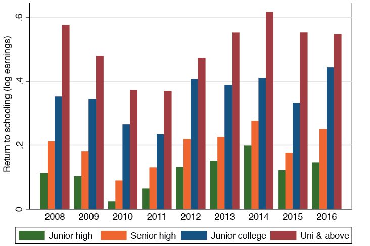
Figure 21.11 Returns to different levels of education, 2008–16

Source: Authors’ own calculation from RUMiC data.

To sum up, there is evidence to suggest there was a structural change between 2010 and 2011 that may have impacted, at least for a while, on experience–earnings profiles and returns to education and, more permanently, on the industry sector of employment.

It is to be expected that the changing mix of jobs in cities will affect the demand for migrant workers, so it would be worthwhile examining this link in more detail. If, however, the changing mix of jobs reduced migration flows so dramatically, it is reasonable to think some evidence of this would be found in a large change in average wage relativities between the home village and the city, but on the basis of our evidence this appears not to be the case.

Wage variation across cities

One potential way to make progress in understanding the relationship between migrant flows and migrant outcomes is to analyse different outcomes across cities and ask why there is such a large variation in migrant earnings between cities and whether this variation has narrowed in response to migration. Do migrants move disproportionately to cities where earnings are highest? These questions are obviously related to the overarching question posed at the beginning of this chapter, which compared city wages with home village wages and asked whether these gaps can be related to changes in net migration to large cities.

In Figure 21.12, we present the earnings variation across our 15 survey cities. There are eight coastal cities (Guangzhou, Shenzhen, Dongguan, Shanghai, Nanjing, Wuxi, Hangzhou and Ningbo) and seven inland cities (Zhengzhou, Luoyang, Hefei, Bengbu, Chongqing, Chengdu and Wuhan). The cross-city earnings variation is calculated after allowing for the different characteristics of migrants in each city. This is done by including city dummy variables in the earnings equations described earlier, with Guangzhou used as the omitted category. Thus, each city’s position is relative to Guangzhou. For example, real monthly earnings in Hefei in 2008—standardising for all personal migrant characteristics included in the regression for each city—were about 18 per cent below Guangzhou’s real monthly earnings.

The data indicate there are large average earnings gaps for migrant workers in different cities, even after standardising for individual personal observable characteristics. The gap across these cities has not narrowed significantly over the past nine years. In 2008, the standard deviation of the city coefficients was about 0.19, while in 2016 it was 0.17. Between the top and bottom earning cities, the earnings gap in 2008 was 0.63 log points, and in 2016 it was 0.58 points.⁵

Figure 21.12 indicates that coastal cities have the highest incomes and inland cities the lowest, and the gap between the two does not seem to have narrowed. In general, cities also maintained their relative positions: Shenzhen and Shanghai maintained their higher incomes and Luoyang and Wuhan remained among the lower income group.

If migration flows are responsive to city wages, they will respond to real wages—that is, wages paid in the city need to be adjusted for city living costs. There are city-level consumer price index (CPI) changes available for each city to adjust for price changes over time, but no official special price indices with which to compare the cost-of-living differentials between cities. Urban economists, therefore, often turn to housing prices as a proxy to measure differing living costs. In addition, other costs may generally be higher in large cities and rent levels do not adequately capture their effect. For example, the larger the city, the higher are the travel costs (both monetary and time) and these may not relate closely to average rent levels.

To explain migration flows, we should also consider the cost of travelling between the home village and the city. Long-distance migration may provide larger monetary gains on arrival, but may involve higher monetary and psychological costs of travel to the city, which may discourage many from migrating to higher-wage regions.

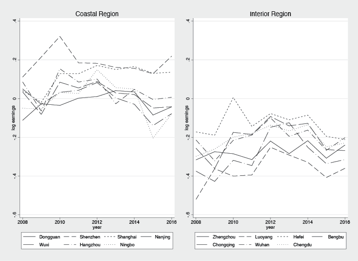
Figure 21.12 City earnings premium relative to Guangzhou, by coastal and inland regions, 2008–16

Source: Authors’ own calculation from RUMiC data.

To gauge the extent to which differing living and mobility costs can explain wage variation across cities, we estimate city-level regressions using the city dummy variable coefficients extracted from estimating migrant earnings equations year by year as the dependent variable (i.e. the coefficients presented in Figure 21.12). We use annual city-level average rent paid by our sample migrants to measure the cost of rent, and use the population size of each city as a proxy for travel and other costs within the city. To explore the relationships between variations of costs of travel to the city and wages, we include in the regressions the proportion of migrants in each city from within the same province. We also include the number of provinces sending to a particular city, excluding the province in which the city is located (the larger the number of sending provinces, the higher is the level of mobility).

It is also possible that city-level wage variations follow government policy guidance. For example, cities where the local government wishes to push out low-profit, labour-intensive firms may set higher minimum wages. We use a direct measure of city-level minimum wages to capture this effect.

Finally, we also use city-level macroeconomic conditions to explain cross-city wage variations. These variables include log per capita gross domestic product (GDP), log per capita exports, the share of migrant workers employed in the manufacturing sector, the share of migrants working in the services sector, together with the city’s secondary industry share in total GDP. Theoretically, if there is perfect labour mobility, city-level macroeconomic conditions should have little to do with city-level wage differentials.

We estimate the regression equation with one variable at a time to indicate associations with cross-city wage levels, and then include all variables in one regression (Table 21.6).

Column 1 in Table 21.6 includes only year dummy variables. Inspection of Figure 21.12 suggests there are no obvious important year-by-year variations of city wage effects and this is confirmed by the low r-squared of 1.3 per cent. The rest of the regressions, however, will control for these year dummy variables.

The next two columns (Columns 2 and 3) show the correlation between city wage variations and the log of city average rent and log of city population. Both variables exert a positive and statistically significant effect. The rent variable alone explains an additional 26.4 per cent of city-level wage variation. The log population explains 4 per cent.

The regression results in Columns 4 and 5 of Table 21.6 indicate that cities with a higher proportion of migrants from within their own province have lower wages, whereas cities with migrants from a larger number of sending provinces have higher wages (54 per cent and 63 per cent of wage variations are associated with variations in the percentage of migrants from the city’s own province and the number of provinces that have sent migrants to the city, respectively). These results suggest migrants are responding to wage signals. High-income cities are attracting migrants from many outside provinces, whereas low-income cities have only migrants from nearby areas (higher intra-province migration).

Column 6 indicates that minimum wages set by local governments are also positively associated with wage variations across cities, explaining 55 per cent of these variations.

The variable that explains most wage variation (78 per cent) is log per capita exports (Column 7). Cities that export more per capita have higher migrant earnings. Log per capita GDP is important to a similar degree—associated with 60 per cent of the wage variations across cities. A city’s industrial structure is also associated with wage variations, though to a much lower extent. The secondary industry share of city GDP within cities is negatively associated with city wages. The share of migrant workers in the manufacturing sector is positively associated while the share of service workers is negatively associated with city wages.

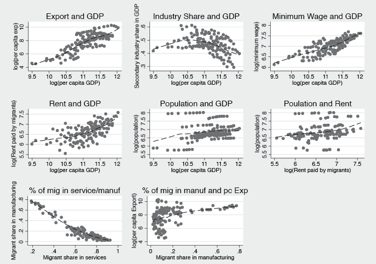
Figure 21.13 Correlations between city-level variables

Source: Authors’ own calculation from RUMiC data.

It is important to understand that these regressions only examine the association between variables and do not estimate causal links between these variables and city-level wage variations. In addition, many right-hand side variables are highly correlated with each other; city per capita exports are highly correlated with city per capita GDP, as is city average rent paid by migrants and city population, and so on. Figure 21.13 presents these interrelationships. With so many multi-collinearities, it is not surprising that when all variables are included many coefficients switch sign and become statistically insignificant (Column 11 of Table 21.6). The dominant variables that remain statistically significant are per capita exports, rent paid by migrants, minimum wages, industry share of GDP, number of sending provinces for each city and migrant share in manufacturing or services. We keep these variables in the last column of Table 21.6.⁶ The total variations in city wages that can be ‘explained’ by the association with these variables is 85 per cent, which is quite high. How, then, should we decide which of these factors dominates?

Following Dickens and Katz (1987), we derive a bounded range for the contribution of these variables. The lower bound is observed by examining the increase in explained variation by adding a particular variable of interest, whereas the upper bound is evaluated by using the variable of interest only in the regression. In our case, we use results in Columns 2–10 as the indication for the upper bound and obtain the lower bound for each variable by taking each variable or group of variables out of the regressions from Columns 11 and 12 to evaluate the difference each variable(s) made to the total adjusted r-squared. The lower bound contribution of the variables is listed in the two last rows of Table 21.6. This exercise shows the most important variable contributing to the variation in city residual wages is log per capita exports. The rest of the variables, despite their statistical significance, have trivial effects in explaining city wage variations.

To summarise the above descriptive analysis, the following points are important. First, although living costs can explain some of the cross-city residual wage variations, the power of explanation is rather small. Second, the signs of the correlation between city wage variation and that of the migrants’ sending region composition seem to suggest that migrants are responsive to wage signals and the higher the wage, the higher is the proportion of migrants from afar. Third, despite the current level of mobility, which is quite high, wage variation across cities is still most strongly correlated with city macroeconomic variables—in particular, the per capita export level. These macroeconomic variables, to a large extent, capture city variations in productivity.

This last point leads us to conclude that although the current level of labour mobility is high, it is not high enough to eliminate the main part of cross-city wage variations. In fact, if only the cost of living variables are included (rent and population size), only 26 per cent of the cross-city residual wage variation can be explained.

Why are cross-city productivities so important? Why hasn’t migration largely removed these macro effects? There could be two reasons for this. The first is that considerable policy-induced mobility restrictions remain, which stop more migrants from moving to higher-earnings cities and reduce relative wages. The second reason is that there are unobservable psychological costs of migration, which are much higher for those moving to higher-earnings cities than those moving to lower-earnings cities. Based on our current data, however, it is unlikely we can separately identify these two causes. In any case, the current policy—which encourages migrants to move to small hometown cities rather than large, more productive cities—should be part of the ‘policy restrictions’ we have in mind.

Table 21.6 City-level regressions

	(1)	(2)	(3)	(4)	(5)	(6)	(7)	(8)	(9)	(10)	(11)	(12)
	Year only	Rent	Population	Percentage of migrants within province	Number of source provinces	Minimum wage	Per capita exports	Per capita GDP	Industry share (services)	Industry share (manuf.)
log(rent)		0.286***									0.098**	0.114***
		[0.043]									[0.037]	[0.034]
Log(popu)			0.070**								–0.013
			[0.029]								[0.015]
Percentage within province				–0.369***							0.007
				[0.031]							[0.035]
Number of source provinces					0.030***						0.005*	0.007***
					[0.002]						[0.003]	[0.003]
log(min_wage)						0.709***					0.164***	0.111**
						[0.058]					[0.059]	[0.056]
log(export_pc)							0.106***				0.059***	0.062***
							[0.005]				[0.010]	[0.009]
log(gdp_pc)								0.313***			0.020
								[0.023]			[0.031]
Secondary industry share									–1.524***	–1.477***	–0.368*	–0.128
									[0.234]	[0.237]	[0.210]	[0.155]
Percentage of migrants in service industry									–0.378***		–0.422***
									[0.074]		[0.121]
Percentage of migrants in manufacturing										0.326***	–0.267**	0.116**
										[0.070]	[0.110]	[0.051]
Year fixed effects	Yes	Yes	Yes	Yes	Yes	Yes	Yes	Yes	Yes	Yes	Yes	Yes
Observations	126	126	126	126	126	126	125	126	126	126	125	125
Adjusted R2	0.0135	0.278	0.0531	0.549	0.621	0.562	0.787	0.614	0.337	0.315	0.864	0.852
Lower bound (11)		0.007	–0.001	–0.002	0.002	0.008	0.034	–0.001	0.014	0.006
Lower bound (12)		0.013			0.009	0.004	0.054			0.006

*** p<0.01, ** p<0.05, * p<0.1

Conclusions

The most important labour reallocation change in China is the slowing growth rate of rural hukou workers moving to large cities and the significant increase in rural hukou workers staying in their hometown to work in nonagricultural jobs. This redirection of labour reallocation does not appear to be a response to a narrowing of the earnings gap between the city and the rural hometown. In fact, the gap between migrant earnings in cities and what they would have earned had they stayed in their rural hometown to work in the nonagricultural sector in 2016 is almost as large as it was in 2008.

Furthermore, we find no evidence of increasing migrant dissatisfaction with life in the city. The proportion of migrants who are happy or very happy is much the same throughout the period. The proportion of migrants who would like to live in the city permanently is also unchanging. These facts lead us to conjecture that the large reduction in rural-to-urban migrants is primarily related to government policy. The economic return from allowing people to move to the city remains high, at least in terms of the wages they can earn.

Among rural-to-urban migrants over the past nine years there have been some large changes in age and gender composition in directions that might be anticipated when migrant inflows slow. It is to be expected that the migrant workforce would age. In 2008, only 23 per cent of men and 19 per cent of women in the workforce were aged 40 and above. By 2016, these ratios increased to 42 per cent for men and 45 per cent for women. Furthermore, a larger proportion of the older labour force comprises women who do not appear to be newcomers as they have been in their current job for more than five years.

As the inflow of new migrants has slowed, and the migrant workers have aged, it is to be expected that increases in the migrant stock’s education would slow. The younger migrant generation is slightly better educated, but the increasing proportion of older migrant workers has low education levels, especially older women. Education improvement is slow. The average education level (measured in years of schooling) over the nine years has increased by less than 0.3 years.

The number of hours worked for both wage earners and the self-employed has not changed much despite the introduction of the New Labour Law, which stipulates that standard work hours should be no more than eight hours daily and no more than 40 hours a week. Work hours far exceed these standards. Wage earners, on average, worked 250 hours monthly and the self-employed worked 330 hours.

Real hourly earnings growth for migrant wage earners continues to grow strongly, although the growth has moderated since 2013, while the self-employed are doing better since 2013 in terms of hourly income. There is, however, no obvious link between these changes and reduced migration inflows.

So what might we expect looking forward? It seems fairly clear that the migration patterns of the post-GFC period will continue, partly because of the changing balance between export markets and internally stimulated growth, but mainly because it appears the slowdown in migration to large cities is primarily the result of policy. We cannot find significant evidence to suggest that the economic incentives for migrants to move to the large cities or their desire to stay in the large cities have declined. Rising agricultural productivity will continue to produce surplus farm labour that needs to find alternative jobs, but these other jobs will be located closer to home since the small city development strategy seems firmly in place.

References

Dickens, W. T. and Katz, L. F. (1987), Inter-industry wage differences and industry characteristics, in K. Lang and J. S. Leonard (eds), Unemployment and the Structure of Labor Markets, Oxford: Basil Blackwell.

Glaeser, E. L. and Gottlieb, J. D. (2008), The economics of place-making policies, Brookings Papers on Economic Activity (1): 155–253. doi.org/10.1353/eca.0.0005.

Glaeser, E. L. and Gottlieb, J. D. (2009), The wealth of cities: Agglomeration economies and spatial equilibrium in the United States, Journal of Economic Literature 47(4): 983–1028. doi.org/10.1257/jel.47.4.983.

Meng, X. (2013), Rural–urban migration, in R. Garnaut, C. Fang and L. Song (eds), China: A new model for growth and development, Canberra: ANU E Press. doi.org/10.22459/CNMGD.07.2013.09.

Meng, X. (2014), China’s labour market tensions and future urbanisation challenges, in R. Garnaut, C. Fang and L. Song (eds), Deepening Reform for China’s Long-Term Growth and Development, Canberra: ANU Press. doi.org/10.22459/DRCLTGD.07.2014.15.

Meng, X. (2017), The Labor Contract Law, macro conditions, self-selection, and labor market outcomes for migrants in China, Asian Economic Policy Review 12(1).

Moretti, E. (2011), Local labor markets, Handbook of Labor Economics 4: 1237–313. doi.org/10.1016/S0169-7218(11)02412-9.

National Bureau of Statistics (NBS) (various years [a]), China Yearbook of Household Survey, Beijing: China Statistics Press.

National Bureau of Statistics (NBS) (various years [b]), China Rural Household Survey Yearbook, Beijing: China Statistics Press.

National People’s Congress (NPC) (2007), Labour Contract Law of the People’s Republic of China, Beijing: NPC. Available from: english.mofcom.gov.cn/aarticle/policyrelease/internationalpolicy/200703/20070304475283.html.

State Council (2014), National New Urbanization Plan (2014–2020), Xinhua News Agency, 16 March. Available from: politics.people.com.cn/n/2014/0317/c1001-24649809.html.

World Bank (2009), China—From Poor Areas to Poor People: China’s Evolving Poverty Reduction Agenda, An Assessment of Poverty and Inequality. World Bank. Available from: documents.worldbank.org/curated/en/816851468219918783/China-From-poor-areas-to-poor-people-Chinas-evolving-poverty-reduction-agenda-an-assessment-of-poverty-and-inequality.

---