10. Changes in human tooth-size and shape with the Neolithic transition in Indo-Malaysia

David Bulbeck

Introduction

During my Master of Arts studies on Holocene human remains from Indonesia and Malaysia, I was the beneficiary of excellent supervision from Colin Groves and the late Alan Thorne. At the time, the general view was that the ‘Mongoloid’ features of most Southeast Asians reflect the late Holocene immigration of their ancestors from Northeast Asia into a region previously inhabited by large-toothed ‘Australoids’ (e.g. Jacob, 1967a; Howells, 1973; Bellwood, 1978). At the same time, Christy Turner was developing an alternative perspective of long-term continuity in Southeast Asia of a ‘Sundadont’ dental morphology complex, distinguished from the ‘Sinodont’ complex of Northeast Asia and the New World by features such as less marked incisor shovelling (e.g. Turner, 1983). Also, some biological anthropologists were developing a model that explained post-Neolithic craniodental changes in terms of biological adaptation to changed selection pressures (e.g. Carlson and van Gerven, 1977). The driving force, according to this model, was the reduced demand on the masticatory apparatus associated with the Neolithic transition, as people now grew crops low in fibrous content, and often cooked their food in pots to soften it further. Hence, my MA thesis proposed that Southeast Asia’s late Holocene transition to smaller teeth and jaws, and broader and less robust crania, reflected local adaptation to the reduced need for large tooth mass (Bulbeck, 1981, 1982).

Colin Groves was very supportive of this ‘Neolithic tooth-size reduction’ model, and indeed highlighted it in his contribution at a major symposium (Groves, 1989). On the other hand, as I belatedly discovered, Loring Brace (1976) had already rejected the model’s applicability for Southeast Asia. Brace accepted it for China, but argued that the retention of larger teeth in Southeast Asia pointed to a later onset of the Neolithic there, attributable, moreover, to immigration from South China (see also Brace and Hinton, 1981). Subsequently, Hirofumi Matsumura produced a series of studies that emphasised morphological similarities between Southwest Pacific and early Southeast Asian cranial remains. A critical aspect was Matsumura’s removal of sheer tooth-size from the comparisons, allowing him to argue that the relative sizes of the different tooth diameters (‘tooth shape’) also pointed to Neolithic immigration from China into Southeast Asia (e.g. Matsumura and Hudson, 2004). These views accorded with a growing consensus amongst historical linguists that the Austroasiatic and Austronesian languages, which dominate Southeast Asia ethnographically, trace their origins to the north.

Other biological anthropologists have presented analyses that support long-term population continuity in Southeast Asia (e.g. Hanihara, 1994; Storm, 1995; Manser, 2005; Demeter, 2006; Pietrusewsky, 2006). However, only Manser’s study found the Neolithic tooth-size reduction model useful. Indeed, Storm instead preferred an alternative explanation of body-size reduction related to post-Pleistocene warming.

The task of this contribution is to rigorously test whether biological adaptations to agriculture, and the use of pottery for cooking, could explain late Holocene craniodental change in Indo-Malaysia – the part of Southeast Asia where my specialisation lies. There are now enough well-dated burial series from Sulawesi, Borneo, Java and Malaya to test two main predictions of the Neolithic tooth-size reduction model:

1. Indo-Malaysian tooth-size should show continual reduction over time, not only between the pre-Neolithic and the Neolithic, but also continuing into the Early Metal Phase (EMP) and modern times.
2. Pre-Neolithic and late Holocene Indo-Malaysians should have similar tooth shape.

Depending on the obtained results, the discussion will also briefly examine the efficacy of tooth-size reduction as a driver for late Holocene change in Indo-Malaysian cranial shape, and review recent insights from human genetic and osteological comparisons.

Materials and methods

The dental metrical analyses presented here include male and bisexual samples. The male analyses cater for the critical Late Pleistocene Java sample, which is exclusively male. The bisexual analyses enable the inclusion of archaeological teeth that are difficult to sex – for instance, loose teeth, and teeth from sub-adults – and also cater for series where both males and females, on their own, are sparsely documented. In these analyses, tooth-size comparisons (but less so shape comparisons – Bulbeck, 1981; Bulbeck et al., 2005) are prone to distortion due to the samples’ variable sex composition, given that male teeth are on average larger than female teeth. However, many of the prehistoric Indo-Malaysian samples are dominated by specimens that cannot be sexed, and so they can be analysed only as bisexual samples.

The present coverage of recent Indo-Malaysian populations focuses on Indonesia and the Orang Asli (‘aboriginal people’) of Malaya, including the Semang ‘Negritos’. Several Southwest Pacific and Northeast Asian samples are also included so as to provide a regional context (Table 10.1). Most of the samples included here are based on dental casts from living subjects or anatomical collections of skulls from persons of known sex. Two exceptions are the ethnohistorical Motu cemetery on Motupore Island, Papua New Guinea (PNG), and the Euston cemetery on the Murray Valley, with an estimated age between 2,000 and 6,000 years ago (Pardoe, 1988). Postcranial material was available to assist sexing the Motupore skulls (Brown, 1978) but sexing of the Euston skulls relied on cranial size and robustness (Brown, 1981). A third exception is the ‘historical Sulawesi’ sample, which mainly comprises geographically dispersed archaeological finds (Table 10.2). Many of these remains cannot be reliably sexed and so the sample is best treated as bisexual.

Table 10.1: Recent/historical samples used in the comparisons.

Sample	Male sample size	Bisexual composition	Source
Shanghai Chinese	14–104	♂ and ♀ about equal	Brace et al. 1984
Historical Sulawesi	Not applicable	More ♂ than ♀ (probably)	See Table 10.2
Jahai Semang, Malaya	13–19	Pooled into Semang sample, more ♂ than ♀	Bulbeck et al. 2005
Batek Semang, Malaya	8–12		Bulbeck et al. 2005
Temiar Senoi, Malaya	6–30	♂ and ♀ about equal	Bulbeck et al. 2005
Temuan, Malaya	9–16	Pooled into Aboriginal Malay sample, ♂ and ♀ about equal	Bulbeck et al. 2005
Semelai, Malaya	14–22		Bulbeck et al. 2005
Batawi, Java	96–139	More ♂ than ♀	Snell 1938
Surabaya Javanese	35–63	Not available	Snell 1938
Motupore Island, PNG	9–11	♂ and ♀ about equal	Brown 1978
Eastern Highlands, PNG	32–53	Not available	Doran and Freedman 1974
Walbiri, Central Australia	29–136	Not used	Barrett et al. 1963, 1964
Euston, Murray Valley	14–27	♂ and ♀ about equal	Brown 1978

Source: All sources listed in the table and cited fully in the references.

Table 10.2: Historical Sulawesi dental metrics.(A)

Tooth	Mesiodistal (MD) diameters			Buccolingual (BL) diameters
	Sample size	Mean	Standard deviation	Sample size	Mean	Standard deviation
Upper medial incisor (I1)	11	8.3	0.90	14	7.2	0.45
Upper lateral incisor (I2)	10	7.3	0.66	13	6.7	0.34
Upper canine (C)	20	7.9	0.54	21	8.2	0.66
Upper first premolar (P3)	28	7.5	0.68	27	9.5	0.90
Upper second premolar (P4)	21	7.2	0.45	21	9.5	0.60
Upper first molar (M1)	23	10.7	0.72	23	11.7	0.59
Upper second molar (M2)	25	9.8	0.69	24	11.8	0.80
Upper third molar (M3)	19	9.4	0.64	19	11.9	0.75
Lower medial incisor (I1)	11	5.8	0.57	12	6.3	0.49
Lower lateral incisor (I2)	16	6.0	0.49	20	6.2	0.42
Lower canine (C)	14	7.3	0.47	16	8.0	0.40
Lower first premolar (P3)	20	7.1	0.46	20	8.1	0.55
Lower second premolar (P4)	24	7.4	0.64	24	8.3	0.61
Lower first molar (M1)	31	11.5	0.57	33	10.8	0.48
Lower second molar (M2)	34	11.3	0.71	35	10.4	0.54
Lower third molar (M3)	25	11.3	0.94	25	10.7	0.75

Note: A. The sample includes teeth dated to the second millennium CE from the Talaud Islands in North Sulawesi (Bulbeck, 1981), teeth from ethnohistorical burials near Lake Towuti in central Sulawesi (laboratory notes), colonial period Bugis skulls (museum notes), seventeenth to twentieth-century Makassar teeth from Batu Ejaya in southwest Sulawesi (Bulbeck, 2004), and teeth from seventeenth to nineteenth century ‘Macassan’ skulls in the Northern Territory (museum notes).

Source: All sources listed in the notes section.

Numerous prehistoric samples from Indo-Malaysia are also available, dating between the Late Pleistocene and the EMP (Table 10.3). Where the sex composition of the bisexual samples could be assessed, they may have more males than females (the Gua Cha samples), approximately equal numbers of males and females (Mesolithic Java, Gilimanuk) or more females than males (the Niah samples). Some of the samples are composite, especially the ‘Early Sulawesi’ sample (Table 10.4). Early Sulawesi, along with Melanta Tutup in Sabah, and Neolithic and EMP Java, lack observations (as placed in the public domain) on some of their tooth diameters. Included for comparison are Khok Phanom Di, Thailand, with burial goods similar to those from Neolithic Malaya (Bellwood, 1993), and the terminal Pleistocene cemetery from Coobool Creek, in Australia’s Murray Valley, for which only buccolingual diameters are available (Brown, 1989).

Table 10.3: Prehistoric samples used in the comparisons.

Site(s)	Location	Age	Comparisons	Data source	Dating source
Khok Phanom Di	Southern Thailand	Neolithic, 4–3.5 ka	Bisexual (♂, ♀ + children)	Tayles 1999	Tayles 1999
See Table 10.4	Early Sulawesi	mid-Holocene	Bisexual	See Table 10.4	See Table 10.4
Leang Buidane	Talauds, North Sulawesi	EMP, 700–1200 CE	Bisexual	Bulbeck 1981	Bellwood 1976
Leang Codong	Southwest Sulawesi	EMP, ~2-1 ka	Bisexual	Jacob 1967a	Bulbeck 1996–97
Pre-Neolithic Niah	Sarawak	20–8 ka	Bisexual	Manser 2005	Manser 2005
Neolithic Niah	Sarawak	Neolithic, 3.5–2 ka	Males, bisexual	Manser 2005	Manser 2005
Melanta Tutup	Sabah	Neolithic/EMP, 3.5-1 ka	Bisexual	Chia et al. 2005	Chia 2008
Gua Cha Hoabinhian	Malaya	mid-Holocene, 7–3 ka	Males, bisexual	Bulbeck 2005a	Bulbeck 2005a
Gua Cha Neolithic	Malaya	Late Neolithic, 3–2 ka	Males, bisexual	Bulbeck 2005a	Bulbeck 2005a
Guar Kepah	Malaya	Transitional Neolithic ~6 ka	Bisexual	Jacob 1967a	Tieng 2010(A)
Gua Harimau	Malaya	Neolithic/EMP, 3-2 ka	Bisexual	Bulbeck 2001	Bulbeck 2001
Wajak, Gua Lawa 1	Java	Pleistocene, ~30-20 ka	Males	Storm 1995; Détroit 2002	Storm et al. in press; Détroit 2002
Mesolithic Java(B)	Java	Pleistocene to mid-Holocene, 13–4 ka	Males, bisexual	Jacob 1967a; Détroit 2002; Noerwidi 2011–12	Jacob 1967a; Détroit 2002
Neolithic Java(C)	Java	Neolithic, 3.5–2.5 ka	Bisexual	Storm 1995; Détroit 2002; Noerwidi 2011–12	Storm 1995; Détroit 2002; Noerwidi 2011-12
EMP Java(D)	Java	~2–1 ka	Bisexual	Snell 1938; Jacob 1964; Noerwidi 2011–12	Jacob 1967a; Noerwidi 2011–12
Gilimanuk	Bali	EMP, 2–1 ka	Bisexual	Jacob 1967b	Anggraeni 1999
Coobool Creek	Murray Valley, Australia	Pleistocene, ~15 ka	Only males used	Brown 1989	Brown 1989

Notes: A. Tieng reports a radiocarbon date on marine shell of 5700 ± 50 BP for the Guar Kepah shell middens. The calibrated date (Intcal 09), allowing a delta R correction of 15 ± 38 (Singapore), would be 5967-6269 BP (2 sigma). The age of the shell middens serves as a maximum age for the burials. Pot sherds from all levels in the middens, and betelnut staining of the burials’ teeth (Bulbeck, 2005b), indicate the burials are Neolithic.

B. Sampung; Pawon; Song Keplek 1 and 4; Song Terus 1; Gua Braholo 1, 4, 5, 7 and /H8.

C. Hoekgroet ♀; Gua Jimbe; Gua Kecil; Song Keplek 5 ♀; Gua Braholo loose teeth; Song Tritis.

D. Puger ♂; Anjar Lor ♀; Batujaya and Plawangan for lower premolars, M1 and M2.

Source: Includes data from all sources listed in the table and cited fully in reference list.

Table 10.4: Early Sulawesi dental metrical data.

Diameter	Leang Buidane Pre-ceramic, Talaud Islands(A)	Gua Mo’o Hono, Lake Towuti(B)	Leang Burung 1 Trench B, southwest Sulawesi(C)	Bola Batu, southwest Sulawesi(D)	Overall average
I1 MD			8.4		8.4
I1 BL			6.8		6.8
C MD	8.2				8.2
C BL	8.9				8.9
P3 MD	8.0				8.0
P3 BL	10.0			8.6	9.3
P4 MD	7.4	8.5		6.5	7.5
P4 BL	9.9	9.3		7.8	9.0
M1 MD	11.95			9.9	11.3
M1 BL	12.3			10.6	11.45
M2 MD	11.3		9.5	10.4	10.6
M2 BL	12.5		11.6	10.0	11.7
I2 MD				6.8	6.8
I2 BL				6.1	6.1
C BL				7.0	7.0
P3 MD				7.0	7.0
P3 BL				7.4	7.4
P4 BL				7.7	7.7
M1 MD				12.3	12.3
M1 BL				11.2	11.2
M2 MD		11.0			11.0
M2 BL		10.15		9.5	9.9
M3 BL				8.4	8.4

Notes: A. Unsexed adolescent stratified beneath the EMP cemetery (Bulbeck, 1981).

B. Teeth from spits 19 to 26, perhaps female, associated with 6–8 ka radiocarbon dates (Bulbeck et al., 2013). Data exclude teeth too worn for even their buccolingual diameters to be recorded.

C. Primary burial, perhaps male, directly radiocarbon dated to 4610 ± 220 BP (Bulbeck, 2004).

D. Slightly mineralised remains, some probably male, from pre-ceramic levels (Bulbeck, 2004).

Source: Includes data from all sources listed in notes and fully cited in reference section.

The statistical application employed in this study is Penrose’s (1954) size and shape statistic, which divides Pearson’s ‘Coefficient of Racial Likeness’ (CRL) into size and shape components. Like the CRL, Penrose’s size and shape statistics are based on calculating a grand standard deviation for all the samples entered for analysis, dividing the samples’ means by this grand standard deviation, and calculating the differences between the standardised means. I have developed an Approach database template that manages these steps, but only for up to 17 samples, which places a limit on how many samples with a reasonable sample size can be included in any analysis. However, I can freely add samples of very small sample size, because their variance would have minimal effect on the grand standard deviation, and so samples like these can be simply entered as mean values to be standardised. (More sophisticated statistical techniques that require individual specimens, with original measurements as observed or estimated for every analysed variable, are inappropriate for this study. This is because the dental metrical data are publicly available mainly in the form of means and standard deviations, and because most samples are dominated by incomplete dentitions or even loose teeth.)

Penrose’s size component has the advantage that, when the calculated statistic is expressed as its square root, it is additive along a single dimension. For instance, if A is x larger than B, and B is y larger than C, then A is (x + y) larger than C. A second advantage is that the size difference tracks the average difference between samples in terms of grand standard deviations. So, for instance, if we assign C a size value of 0 (being smallest), and we then compute B’s size as 0.5 and A’s size as 1.0, we can state that A is on average one standard deviation larger than C, while B is half a standard deviation from both A and C.

Penrose’s shape component essentially captures the variance that cannot be attributed to size. To make the shape distances more intuitive, two transformations are performed here. The first transformation is to express the calculated shape distances as their square roots, to convert them to Euclidean distances. The second transformation involves dividing each inter-sample shape distance by the square root of the product (or geometric average) of the average shape distances of the two samples being compared. For instance, if A has an average shape distance of 0.4 from the other samples, and B an average shape distance of 1.6, and their shape distance from each other is 0.8, their transformed (calibrated) shape distance would be 0.8/0.8 (the geometric average of 0.4 and 1.6), or 1. A value of 1 can be thought of as the ‘expected’ shape distance between any two samples, while values less than 1 (greater than 1) reflect cases of samples that are more similar (less similar) in shape than would be expected. In addition to relating shape differences to a benchmark of 1, this calibration process enables relatively small shape distances between a pair of samples to stand out, whether these samples’ shape distances are on average large or small. (This calibration process also accommodates shape distances computed from different selections of variables in the same analysis, as later described for the analysis concerned.)

To present an overall view of the obtained shape distances, the samples are clustered into dendrograms using average linkage. In addition, two refinements are included, to the degree permitted by the dendrogram structure. (The calculations, performed using Excel spreadsheets, are available from the author on request.)

The first refinement involves seriating the samples along a single dimension. The samples most unlike each other are placed at the two extremes, and the other samples are positioned to the degree that they approach one or the other extreme. The success of the seriation can be calculated as the coefficient of variation between the seriated distances and the most similar, perfect seriation of those distances (see footnotes to Tables 10.5 to 10.8).

The second refinement is to vary the dendrogram’s branch lengths according to the represented distances. A long branch in the dendrogram reflects a considerable shape disjunction, and a sample that accumulates great branch length with respect to the analysed samples’ final joining distance (represented as 0 in the dendrogram) stands out as generally different from the other samples. The distance between any two samples is represented by the minimum horizontal distance that has to be traversed in tracing a path, through the dendrogram, that connects the two samples. How successful the traversed horizontal distances are in representing the shape distances can also be calculated in terms of their coefficient of variation. (The algorithm to calculate branch lengths is based on the average within-distance compared with the average outside-distance. For instance, if A and B cluster together at a distance of 0.5, but A is 0.1 farther from the other samples than B is, then the stem length of A is calculated as 0.5/2 + 0.1/2 = 0.3, while the stem length of B is calculated as 0.5/2 – 0.1/2 = 0.2.)

Five Penrose size and shape analyses are presented here. The first includes all of the male samples for all tooth diameters. The second analysis also focuses on male samples but is restricted to buccolingual diameters. Buccolingual diameters are not susceptible to reduction through interstitial wear, whereas, when mesiodistal diameters are included, there is a risk that the calculated size and shape distances mainly reflect differences in interstitial wear rates (but see Results). The third analysis includes the bisexual samples for all tooth diameters. The fourth comparison focuses on the same bisexual samples, but only on their buccolingual diameters, for the same reason as with the second analysis. Finally, the fifth analysis includes the four prehistoric Indo-Malaysian samples that are lacking data for some of the tooth diameters (see Results section).

Principal Components Analysis (PCA) was also undertaken of all of the analyses presented here, with the sample means submitted to PCA. In each case, the first principle component captured size, as would be expected of biological data (Joliffe 2002). The implications barely differ from the implications of the Penrose size analyses, and so it would be redundant to also present the PCA size results. After the 45–84% of variance accounted for by size was removed, the second, third and other principle components captured a maximum of 15% of variance. In most cases, this was too low to allow for ready interpretation. Accordingly, the PCA results are excluded from this contribution.

Results

First analysis: 17 male samples, all 32 diameters

The Penrose size comparisons are presented at the top of Figure 10.1 (Figure 10.1a). The results would be consistent with a scenario of pronounced tooth-size reduction in Indo-Malaysia between the Pleistocene and early Holocene, with continuing tooth-size reduction during the Neolithic and recent times. Surabaya males from Java show the smallest teeth, whereas the Late Pleistocene Java sample has the largest teeth, on average 2.3 standard deviations larger than Surabaya Javanese. The two pre-Neolithic Indo-Malaysian samples have larger teeth than the two Neolithic Indo-Malaysian samples, whose teeth are of above average size by recent Indo-Malaysian standards. Also of interest, Shanghai Chinese, and the Motupore males from Papua New Guinea, both resemble recent Indo-Malaysians in their tooth-size, whereas the other three Southwest Pacific samples have teeth that are much larger.

The Penrose shape distances (square roots) are presented at Table 10.5, both before and after calibration. The order of the samples reflects their order after seriation of the average-linkage dendrogram, which is illustrated in Figure 10.2. As shown there, the recent Southwest Pacific samples are all placed at one half of the seriated order and the recent Indo-Malaysian (and Chinese) samples toward the other half. Thus, seriation of the dendrogram appears to identify a distinction between ‘Australoids’ and ‘Mongoloids’ in their tooth shape, with the two Semang Negrito samples intermediate between the Australoids and the Mongoloids. The only Indo-Malaysian samples that cluster with the Australoids are the pre-Neolithic samples, including Pleistocene Java. The Neolithic samples, for their part, fall at the polar opposite from the Australoids. This result is consistent with the conventional wisdom (e.g. Bellwood, 1997) of a pre-Neolithic occupation of Indo-Malaysia by Australoid foragers, prior to the immigration of newcomers who introduced the Neolithic to the region.

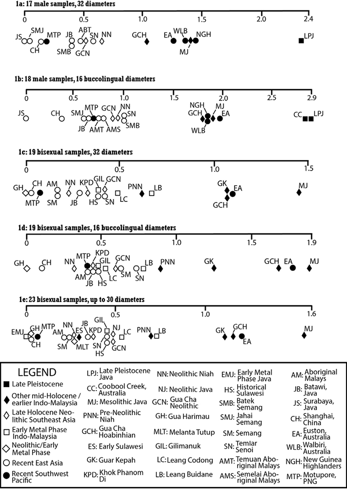
Figure 10.1: Dental metrics, Penrose size statistics comparisons.

Sources: Snell 1938; Barrett et al. 1963, 1964; Jacob 1964; Jacob 1967a, 1967b; Doran and Freedman 1974; Brown 1978; Bulbeck 1981; Brace et al. 1984; Brown 1989; Tayles 1989; Storm 1995; Bulbeck 2001; Détroit 2002; Bulbeck 2004; Bulbeck 2005a; Bulbeck et al. 2005; Chia et al. 2005; Manser 2005; Noerwidi 2011–12; Bulbeck et al. 2013; this paper.

Table 10.5: First analysis: Square roots of Penrose shape distances (top right) and after calibration and seriation (bottom left).(A)

Sam-ple(B)	LPJ	EA	GCH	MJ	NGH	WLB	MTP	SMJ	SMB	SN	AMS	AMT	CH	JB	JS	GCN	NN
LPJ		0.832	0.681	0.807	0.611	0.667	0.568	0.730	0.773	0.757	0.782	0.860	0.688	0.722	0.850	0.937	0.976
EA	1.073		0.565	0.586	0.744	0.585	0.726	0.911	0.854	0.911	0.744	0.837	0.768	0.747	0.977	0.842	0.925
GCH	0.945	0.771		0.657	0.628	0.528	0.544	0.785	0.749	0.738	0.655	0.700	0.629	0.617	0.850	0.694	0.835
MJ	1.113	0.819	1.014		0.590	0.530	0.674	0.766	0.715	0.731	0.586	0.625	0.671	0.585	0.811	0.677	0.899
NGH	0.956	1.144	1.039	1.010		0.332	0.410	0.537	0.575	0.499	0.388	0.482	0.413	0.417	0.560	0.621	0.756
WLB	1.064	0.917	0.892	0.933	0.631		0.432	0.566	0.563	0.491	0.326	0.432	0.373	0.384	0.632	0.621	0.761
MTP	0.887	1.113	0.898	1.106	0.762	0.820		0.479	0.501	0.446	0.461	0.530	0.420	0.431	0.591	0.583	0.815
SMJ	1.046	1.282	1.190	1.133	0.917	0.986	0.818		0.297	0.411	0.563	0.608	0.605	0.599	0.758	0.635	0.982
SMB	1.121	1.218	1.151	1.075	0.995	0.993	0.866	0.470		0.472	0.539	0.564	0.592	0.561	0.743	0.569	0.914
SN	1.147	1.356	1.183	1.145	0.900	0.904	0.799	0.681	0.791		0.372	0.392	0.521	0.441	0.567	0.554	0.860
AMS	1.269	1.187	1.124	1.005	0.751	0.643	0.890	0.998	0.967	0.698		0.276	0.366	0.294	0.483	0.446	0.692
AMT	1.348	1.289	1.162	1.049	0.900	0.823	0.989	1.042	0.978	0.709	0.534		0.380	0.273	0.417	0.447	0.711
CH	1.095	1.201	1.060	1.147	0.783	0.721	0.795	1.051	1.041	0.956	0.719	0.722		0.252	0.402	0.530	0.673
JB	1.186	1.206	1.071	1.019	0.815	0.767	0.843	1.074	1.019	0.837	0.596	0.536	0.502		0.317	0.473	0.673
JS	1.218	1.375	1.288	1.220	0.956	1.101	1.008	1.185	1.176	0.937	0.854	0.713	0.697	0.568		0.592	0.693
GCN	1.368	1.209	1.073	1.041	1.080	1.103	1.013	1.013	0.918	0.934	0.806	0.779	0.939	0.864	0.943		0.629
NN	1.251	1.166	1.133	1.200	1.155	1.187	1.243	1.374	1.294	1.272	1.097	1.089	1.045	1.078	0.969	0.896

Notes: A. The seriated calibrated distances, in the bottom-left half-matrix, show a tendency to be smallest along the diagonal and to increase with each step away from the diagonal, moving horizontally or vertically. In a perfect seriation, with each horizontal or vertical step away from the diagonal, the distances would increase (or at least stay the same). Therefore, the distances shown here were rearranged into the closest perfect seriation that could be found, and the coefficient of variation (68.8%) calculated between the distances shown here and the rearranged distances.

B. LPJ=Late Pleistocene Java; EA=Euston, Australia; GCH=Gua Cha Hoabinhian; MJ=Mesolithic Java; NGH=New Guinea Highlanders; WLB=Walbiri, Australia; MTP=Motupore Island, PNG; SMJ=Jahai Semang; SMB=Batek Semang; SN=Temiar Senoi; AMS=Semelai Aboriginal Malays; AMT=Temuan Aboriginal Malays; CH=Shanghai, China; JB=Batawi, Java; JS=Surabaya, Java; GCN=Gua Cha Neolithic; NN=Neolithic Niah.

Sources: Snell 1938; Barrett et al. 1963, 1964; Jacob 1967a; Doran and Freedman 1974; Brown 1978; Brace et al. 1984; Storm 1995; Détroit 2002; Bulbeck 2005a; Bulbeck et al. 2005; Manser 2005; Noerwidi 2011–12.

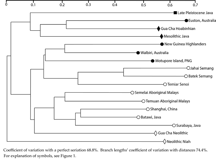
Figure 10.2: Dental metrics, Penrose shape distances, 17 male samples, 32 diameters, seriated average-linkage dendrogram.

Sources: Snell 1938; Barrett et al. 1963, 1964; Jacob 1967a; Doran and Freedman 1974; Brown 1978; Brace et al. 1984; Storm 1995; Détroit 2002; Bulbeck 2005a; Bulbeck et al. 2005; Manser 2005; Noerwidi 2011–12.

Second analysis: 18 male samples, 16 buccolingual diameters

The Penrose size comparisons are presented at Figure 10.1b. The results essentially echo those obtained for males using all diameters, with a clear indication of continual tooth-size reduction in Indo-Malaysia from the Pleistocene through the early Holocene, into the Neolithic and recent times. However, the inclusion of Coobool Creek (Late Pleistocene Australia) in the comparison offers two additional insights. First, the Coobool Creek teeth are larger than those of Holocene Australian Aborigines, as emphasised by Brown (1989). Secondly, Pleistocene Java and Australian teeth appear very similar in size, just as Mesolithic Java tooth-size appears very similar to Holocene Australian tooth-size.

Table 10.6: Second analysis: Square roots of Penrose shape distances (top right) and after calibration and seriation (bottom left).(A)

Sam-ple(B)	CC	EA	MJ	GCH	WLB	AMS	AMT	SN	CH	JB	MTP	JS	NN	GCN	NGH	SMB	SMJ	LPJ
CC		0.501	0.624	0.696	0.582	0.623	0.709	0.857	0.673	0.708	0.833	0.856	0.842	0.904	0.850	0.917	0.940	0.828
EA	0.686		0.561	0.656	0.464	0.591	0.651	0.805	0.655	0.603	0.756	0.746	0.825	0.869	0.723	0.877	0.880	0.767
MJ	0.935	0.875		0.690	0.464	0.467	0.522	0.575	0.558	0.487	0.604	0.608	0.748	0.669	0.536	0.643	0.614	0.570
GCH	1.058	1.038	1.196		0.516	0.526	0.438	0.577	0.450	0.360	0.479	0.423	0.535	0.650	0.630	0.747	0.755	0.551
WLB	0.976	0.811	0.888	1.002		0.274	0.290	0.433	0.359	0.348	0.457	0.483	0.584	0.611	0.402	0.532	0.552	0.577
AMS	1.064	1.052	0.911	1.038	0.597		0.267	0.333	0.379	0.341	0.404	0.425	0.506	0.447	0.392	0.534	0.542	0.605
AMT	1.228	1.174	1.031	0.877	0.642	0.600		0.302	0.318	0.284	0.318	0.360	0.483	0.465	0.421	0.503	0.533	0.586
SN	1.386	1.356	1.062	1.079	0.896	0.700	0.644		0.443	0.368	0.406	0.384	0.551	0.466	0.432	0.544	0.494	0.557
CH	1.171	1.186	1.107	0.906	0.797	0.858	0.730	0.949		0.252	0.255	0.334	0.450	0.441	0.448	0.426	0.446	0.494
JB	1.276	1.131	1.001	0.750	0.801	0.799	0.675	0.818	0.600		0.239	0.192	0.433	0.450	0.395	0.506	0.497	0.413
MTP	1.429	1.350	1.181	0.949	1.002	0.901	0.718	0.859	0.580	0.562		0.177	0.427	0.408	0.382	0.463	0.466	0.518
JS	1.457	1.323	1.182	0.834	1.050	0.940	0.807	0.805	0.752	0.449	0.394		0.391	0.426	0.391	0.537	0.513	0.457
NN	1.268	1.294	1.284	0.931	1.124	0.990	0.958	1.023	0.898	0.894	0.839	0.763		0.447	0.584	0.642	0.716	0.687
GCN	1.383	1.385	1.167	1.149	1.194	0.890	0.938	0.878	0.893	0.944	0.816	0.845	0.784		0.509	0.501	0.581	0.698
NGH	1.371	1.216	0.987	1.175	0.828	0.822	0.895	0.858	0.959	0.875	0.804	0.819	1.081	1.091		0.450	0.446	0.506
SMB	1.394	1.388	1.115	1.312	1.033	1.056	1.007	1.019	0.858	1.055	0.919	1.057	1.119	0.901	0.841		0.280	0.558
SMJ	1.426	1.390	1.063	1.325	1.070	1.069	1.066	0.924	0.895	1.035	0.923	1.008	1.245	0.885	0.832	0.491		0.530
LPJ	1.245	1.201	0.979	0.958	1.108	1.183	1.162	1.032	0.983	0.852	1.017	0.892	1.184	1.223	0.935	0.971	0.921

Notes: A. The seriated calibrated distances, in the bottom-left half-matrix, show a tendency to be smallest along the diagonal and to increase with each step away from the diagonal, moving horizontally or vertically. In a perfect seriation, with each horizontal or vertical step away from the diagonal, the distances would increase (or at least stay the same). Therefore, the distances shown here were rearranged into the closest perfect seriation that could be found, and the coefficient of variation (73.2%) calculated between the distances shown here and the rearranged distances.

B. CC=Coobool Creek; EA=Euston, Australia; MJ=Mesolithic Java; GCH=Gua Cha Hoabinhian; WLB=Walbiri, Australia; AMS=Semelai Aboriginal Malays; AMT=Temuan Aboriginal Malays; SN=Temiar Senoi; CH=Shanghai, China; JB=Batawi, Java; MTP=Motupore Island, PNG; JS=Surabaya, Java; NN=Neolithic Niah; GCN=Gua Cha Neolithic; NGH=New Guinea Highlanders; SMB=Batek Semang; SMJ=Jahai Semang; LPJ=Late Pleistocene Java.

Sources: Snell 1938; Barrett et al. 1964; Jacob 1967a; Doran and Freedman 1974; Brown 1978; Brace et al. 1984; Brown 1989; Storm 1995; Détroit 2002; Bulbeck 2005a; Bulbeck et al. 2005; Manser 2005; Noerwidi 2011–12.

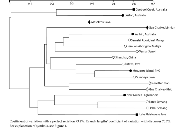
Figure 10.3: Dental metrics, Penrose shape distances, 18 male samples, 16 buccolingual diameters, seriated average-linkage dendrogram.

Sources: Snell 1938; Barrett et al. 1964; Jacob 1967a; Doran and Freedman 1974; Brown 1978; Brace et al. 1984; Brown 1989; Storm 1995; Détroit 2002; Bulbeck 2005a; Bulbeck et al. 2005; Manser 2005; Noerwidi 2011–12.

However, when the calibrated shape distances (Table 10.6) are clustered and seriated, the results differ from Figure 10.2 (the first analysis). The Southwest Pacific samples now split between Australian samples (including Coobool Creek) at one half of the seriation, and New Guinea samples at the other half of the seriation (Figure 10.3). Mesolithic Java and Gua Cha Hoabinhians align with the Australian samples, whereas Late Pleistocene Java takes up a polar position away from Australians. There is however one concordance between Figures 10.2 and 10.3: the two Neolithic samples fall closer to recent Indo-Malaysians than to the pre-Neolithic Indo-Malaysian samples.

The similarity between Australian and New Guinea samples in Figure 10.2, lacking from Figure 10.3, suggests the existence of a ‘Southwest Pacific tooth shape’ based on mesiodistal diameters and their relation to buccolingual diameters. This similarity cannot be attributed to interstitial wear. The Euston Aboriginal teeth were affected by much greater interstitial wear than the Motupore teeth (personal observation). Hence, if interstitial wear were at stake, any Euston-Motupore similarity should be evident in Figure 10.3, not Figure 10.2 – the reverse of what we find. Accordingly, the dentition as a whole apparently reflects a genetically based difference between ‘Australoids’ and ‘Mongoloids’, detectable notwithstanding differences between populations in their interstitial wear rates.

Third analysis: 19 bisexual samples, all 32 diameters

In the Penrose size comparisons (Figure 10.1c), the Neolithic/EMP sample from Gua Harimau shows the smallest teeth. The Niah samples also appear relatively small-toothed, with Neolithic Niah smaller than Neolithic Gua Cha, and pre-Neolithic Niah smaller than Gua Cha Hoabinhians and Mesolithic Java. This however may be affected by the greater representation of females than males in the Niah samples. Another complication is that the Guar Kepah sample, while qualifying as Neolithic, is of similar mid-Holocene antiquity to the Gua Cha Hoabinhians, and indeed their teeth are similarly large. The late Holocene Neolithic samples, for their part, tend to have slightly smaller teeth than the EMP samples. For all that, we can safely conclude that mid-Holocene and earlier Indo-Malaysian teeth appear to have been larger than their late Holocene counterparts.

The shape distances (Table 10.7), upon analysis, produce a pattern similar to that observed for the male samples with all 32 diameters included. The top half of the dendrogram (Figure 10.4) features Southwest Pacific samples, along with mid-Holocene and earlier Indo-Malaysian samples, as well as the Semang and Temiar Senoi from Malaya. The bottom half of the dendrogram includes recent Indo-Malaysians (except the Semang and Senoi), Shanghai Chinese and the late Holocene prehistoric samples. The extreme examples are Gua Harimau and Neolithic Niah, whereas Neolithic Gua Cha now tends towards the middle of the dendrogram. The simplest interpretation of Figure 10.4 may be that it points to broadly ‘Australoid’ (Euston Aborigines to Motupore) and ‘Mongoloid’ (Gua Harimau to Aboriginal Malay) groupings, with pre-Neolithic Niah, Guar Kepah and Gua Cha Neolithic intermediate.

Table 10.7: Third analysis: Square roots of Penrose shape distances (top right) and after calibration and seriation (bottom left).(A)

Sam-ple(B)	EA	GCH	MJ	SM	SN	MTP	PNN	GK	GCN	AM	JB	CH	KPD	LB	LC	GIL	HS	NN	GH
EA		0.558	0.627	0.903	0.872	0.795	0.705	0.896	0.821	0.768	0.791	0.824	0.886	0.836	0.909	0.845	0.856	0.934	1.015
GCH	0.757		0.591	0.730	0.672	0.615	0.465	0.675	0.657	0.605	0.603	0.673	0.703	0.651	0.663	0.660	0.670	0.776	0.875
MJ	0.875	0.924		0.614	0.586	0.602	0.580	0.633	0.518	0.529	0.535	0.616	0.628	0.578	0.641	0.609	0.669	0.806	0.837
SM	1.248	1.130	0.977		0.389	0.473	0.637	0.606	0.577	0.464	0.545	0.550	0.593	0.575	0.699	0.661	0.702	0.758	0.947
SN	1.315	1.134	1.017	0.669		0.463	0.544	0.589	0.454	0.291	0.388	0.502	0.476	0.463	0.509	0.459	0.545	0.627	0.765
MTP	1.174	1.017	1.024	0.797	0.851		0.550	0.543	0.526	0.423	0.422	0.412	0.482	0.512	0.581	0.529	0.609	0.642	0.826
PNN	1.091	0.805	1.032	1.122	1.046	1.037		0.539	0.469	0.389	0.360	0.449	0.504	0.460	0.402	0.414	0.481	0.543	0.640
GK	1.333	1.123	1.084	1.027	1.089	0.983	1.022		0.483	0.482	0.448	0.371	0.360	0.370	0.449	0.464	0.535	0.557	0.872
GCN	1.303	1.168	0.947	1.044	0.896	1.017	0.949	0.940		0.362	0.322	0.422	0.454	0.339	0.412	0.325	0.446	0.460	0.615
AM	1.276	1.126	1.013	0.879	0.602	0.855	0.824	0.982	0.788		0.246	0.332	0.326	0.353	0.382	0.313	0.464	0.515	0.661
JB	1.360	1.162	1.060	1.069	0.829	0.884	0.789	0.946	0.725	0.579		0.260	0.295	0.256	0.273	0.264	0.331	0.450	0.587
CH	1.337	1.223	1.151	1.016	1.012	0.814	0.929	0.738	0.896	0.739	0.599		0.237	0.294	0.361	0.352	0.403	0.514	0.724
KPD	1.410	1.252	1.150	1.076	0.943	0.934	1.022	0.702	0.946	0.710	0.665	0.504		0.323	0.345	0.359	0.413	0.515	0.725
LB	1.372	1.195	1.092	1.076	0.946	1.023	0.962	0.743	0.727	0.794	0.596	0.644	0.694		0.298	0.346	0.327	0.455	0.679
LC	1.363	1.192	1.131	1.215	0.921	1.040	0.851	0.918	0.687	0.692	0.605	0.759	0.760	0.754		0.281	0.354	0.438	0.574
GIL	1.451	1.185	1.178	1.273	1.010	1.130	0.818	0.879	0.861	0.834	0.619	0.770	0.722	0.642	0.596		0.419	0.459	0.632
HS	1.423	1.247	1.281	1.330	1.126	1.232	1.020	1.091	0.970	0.959	0.720	0.827	0.900	0.735	0.925	0.774		0.478	0.594
NN	1.350	1.256	1.341	1.249	1.128	1.131	1.001	0.988	0.871	1.021	0.923	0.993	0.976	0.890	0.883	0.833	0.947		0.517
GH	1.311	1.265	1.244	1.394	1.229	1.299	1.053	1.382	1.040	1.170	1.075	1.251	1.229	1.186	1.086	0.976	1.052	0.797

Notes: A. The seriated calibrated distances, in the bottom-left half-matrix, show a tendency to be smallest along the diagonal and to increase with each step away from the diagonal, moving horizontally or vertically. In a perfect seriation, with each horizontal or vertical step away from the diagonal, the distances would increase (or at least stay the same). Therefore, the distances shown here were rearranged into the closest perfect seriation that could be found, and the coefficient of variation (76.0%) calculated between the distances shown here and the rearranged distances.

B. EA=Euston, Australia; GCH=Gua Cha Hoabinhian; MJ=Mesolithic Java; SM=Semang; SN=Temiar Senoi; MTP=Motupore Island, PNG; PNN=pre-Neolithic Niah; GK=Guar Kepah; GCN=Gua Cha Neolithic; AM=Aboriginal Malays; JB=Batawi, Java; CH=Shanghai, China; KPD=Khok Phanom Di; LB=Leang Buidane; LC=Leang Codong; GIL=Gilimanuk; HS=Historical Sulawesi; NN=Neolithic Niah; GH=Gua Harimau.

Sources: Snell 1938; Barrett et al. 1963, 1964; Jacob 1964; Jacob 1967a, 1967b; Doran and Freedman 1974; Brown 1978; Bulbeck 1981; Brace et al. 1984; Tayles 1989; Storm 1995; Bulbeck 2001; Détroit 2002; Bulbeck 2004; Bulbeck 2005a; Bulbeck et al. 2005; Chia et al. 2005; Manser 2005; Noerwidi 2011–12; Bulbeck et al. 2013; this paper.

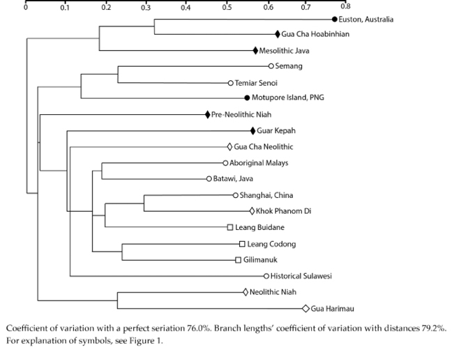
Figure 10.4: Dental metrics, Penrose shape distances, 19 bisexual samples, 32 diameters, seriated average-linkage dendrogram.

Sources: Snell 1938; Barrett et al. 1963, 1964; Jacob 1964; Jacob 1967a, 1967b; Doran and Freedman 1974; Brown 1978; Bulbeck 1981; Brace et al. 1984; Tayles 1989; Storm 1995; Bulbeck 2001; Détroit 2002; Bulbeck 2004; Bulbeck 2005a; Bulbeck et al. 2005; Chia et al. 2005; Manser 2005; Noerwidi 2011–12; Bulbeck et al. 2013; this paper.

Fourth analysis: 19 bisexual samples, 16 buccolingual diameters

When the Penrose size distances for bisexual samples are limited to buccolingual diameters, the resulting graph (Figure 10.1d) can be viewed as a clarification of Figure 10.1c. There is now no overlap in tooth-size between the late Holocene and the mid-Holocene and earlier samples. Moreover, the lack of a systematic size distinction, comparing the Neolithic, EMP and recent/historical samples with each other, is very apparent. (The small size of the Gua Harimau teeth is even more apparent than in Figure 10.1c.)

The structure of the shape distances (Table 10.8; Figure 10.5) is difficult to interpret. The extreme positions of the seriated dendrogram are taken up by Euston Aborigines and Gua Harimau, as in the third analysis. However, the three pre-Neolithic Indo-Malaysian samples now split between Mesolithic Java, which clusters with Euston Aborigines, and pre-Neolithic Niah and Gua Cha Hoabinhians, which seriate adjacently to Gua Harimau. The Neolithic samples (including Guar Kepah) lie in the same half of the dendrogram as Mesolithic Java.

Table 10.8: Fourth analysis: Square roots of Penrose shape distances (top right) and after calibration and seriation (bottom left).(A)

Sam-ple(B)	EA	MJ	SM	GK	CH	KPD	MTP	NN	GCN	LB	SN	AM	GIL	JB	LC	HS	PNN	GCH	GH
EA		0.596	0.820	0.792	0.612	0.589	0.753	0.738	0.721	0.632	0.684	0.509	0.620	0.553	0.636	0.635	0.594	0.613	0.855
MJ	0.992		0.460	0.552	0.447	0.424	0.561	0.688	0.506	0.470	0.496	0.421	0.584	0.454	0.507	0.591	0.581	0.670	0.780
SM	1.370	0.849		0.334	0.357	0.445	0.436	0.607	0.437	0.398	0.479	0.469	0.573	0.500	0.535	0.644	0.595	0.709	0.911
GK	1.374	1.058	0.644		0.289	0.329	0.351	0.493	0.432	0.389	0.494	0.455	0.477	0.429	0.489	0.580	0.589	0.618	0.908
CH	1.193	0.963	0.772	0.650		0.161	0.298	0.442	0.370	0.284	0.403	0.314	0.386	0.271	0.351	0.421	0.468	0.501	0.751
KPD	1.153	0.918	0.967	0.743	0.409		0.326	0.435	0.389	0.310	0.370	0.287	0.332	0.249	0.313	0.397	0.499	0.502	0.714
MTP	1.382	1.138	0.887	0.742	0.708	0.778		0.282	0.365	0.371	0.441	0.370	0.419	0.320	0.414	0.547	0.525	0.590	0.680
NN	1.304	1.344	1.189	1.004	1.011	0.998	0.607		0.419	0.396	0.477	0.418	0.404	0.331	0.398	0.506	0.523	0.556	0.567
GCN	1.334	1.036	0.897	0.921	0.887	0.936	0.823	0.911		0.272	0.310	0.327	0.373	0.337	0.413	0.458	0.540	0.564	0.682
LB	1.232	1.013	0.862	0.874	0.717	0.786	0.883	0.906	0.652		0.349	0.330	0.391	0.239	0.317	0.350	0.480	0.470	0.678
SN	1.264	1.012	0.981	1.051	0.964	0.888	0.991	1.033	0.703	0.834		0.272	0.310	0.329	0.320	0.459	0.497	0.574	0.689
AM	0.998	0.911	1.020	1.026	0.797	0.730	0.884	0.961	0.788	0.836	0.654		0.263	0.267	0.326	0.462	0.406	0.496	0.672
GIL	1.160	1.058	1.190	1.028	0.936	0.809	0.956	0.887	0.858	0.948	0.711	0.640		0.313	0.296	0.460	0.415	0.420	0.706
JB	1.139	1.032	1.142	1.018	0.723	0.667	0.803	0.800	0.852	0.636	0.830	0.715	0.800		0.191	0.317	0.357	0.374	0.567
LC	1.240	1.092	1.156	1.098	0.887	0.794	0.983	0.911	0.989	0.799	0.766	0.826	0.716	0.508		0.326	0.349	0.377	0.577
HS	1.122	1.154	1.264	1.182	0.963	0.912	1.179	1.050	0.994	0.802	0.994	1.062	1.010	0.766	0.746		0.504	0.415	0.604
PNN	1.037	1.121	1.152	1.185	1.057	1.132	1.117	1.071	1.157	1.085	1.064	0.922	0.900	0.851	0.789	1.031		0.297	0.683
GCH	1.037	1.252	1.332	1.205	1.098	1.105	1.217	1.104	1.174	1.031	1.191	1.092	0.883	0.866	0.825	0.824	0.582		0.717
GH	1.247	1.257	1.474	1.527	1.418	1.354	1.209	0.971	1.222	1.280	1.231	1.274	1.279	1.130	1.089	1.034	1.154	1.175

Notes: A. The seriated calibrated distances, in the bottom-left half-matrix, show a tendency to be smallest along the diagonal and to increase with each step away from the diagonal, moving horizontally or vertically. In a perfect seriation, with each horizontal or vertical step away from the diagonal, the distances would increase (or at least stay the same). Therefore, the distances shown here were rearranged into the closest perfect seriation that could be found, and the coefficient of variation (66.1%) calculated between the distances shown here and the rearranged distances.

B. EA=Euston, Australia; MJ=Mesolithic Java; SM=Semang; GK=Guar Kepah; CH=Shanghai, China; KPD=Khok Phanom Di; MTP=Motupore Island, PNG; NN=Neolithic Niah; GCN=Gua Cha Neolithic; LB=Leang Buidane; SN=Temiar Senoi; AM=Aboriginal Malays; GIL=Gilimanuk; JB=Batawi, Java; LC=Leang Codong; HS=Historical Sulawesi; PNN=pre-Neolithic Niah; GCH=Gua Cha Hoabinhian; GH=Gua Harimau.

Sources: Snell 1938; Barrett et al. 1964; Jacob 1967a, 1967b; Doran and Freedman 1974; Brown 1978; Bulbeck 1981; Brace et al. 1984; Tayles 1989; Storm 1995; Bulbeck 2001; Détroit 2002; Bulbeck 2004; Bulbeck 2005a; Bulbeck et al. 2005; Manser 2005; Noerwidi 2011–12.

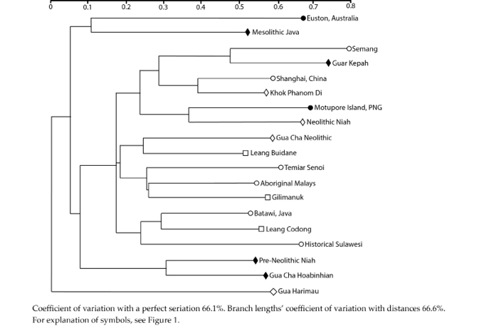
Figure 10.5: Dental metrics, Penrose shape distances, 19 bisexual samples, 16 buccolingual diameters, seriated average-linkage dendrogram.

Sources: Snell 1938; Barrett et al. 1964; Jacob 1967a, 1967b; Doran and Freedman 1974; Brown 1978; Bulbeck 1981; Brace et al. 1984; Tayles 1989; Storm 1995; Bulbeck 2001; Détroit 2002; Bulbeck 2004; Bulbeck 2005a; Bulbeck et al. 2005; Manser 2005; Noerwidi 2011–12.

Fifth analysis: 23 bisexual samples, up to 32 diameters

The fifth analysis has the complication that it includes four samples lacking data for some of the diameters. The available data for these samples cover 30 diameters (EMP Java), 24 diameters (Neolithic Java and Melanta Tutup) and 23 diameters (Early Sulawesi). Further, when these samples are compared with each other, the number of diameters they have in common may be further reduced, to as few as 16 (Neolithic Java compared with Melanta Tutup). The approach adopted here to missing data is to base the pair-wise comparisons on as many diameters as there are data available.

For the size comparisons, each of the additional four samples was individually compared with the 19 samples (those in the third analysis) on all of the diameters for which the individual sample has data. Of these, EMP Java was found to have smaller teeth than Gua Harimau. Therefore, with EMP Java established as the new ‘ground zero’ for the size comparisons, the tooth-size of the other samples is represented by their distance from EMP Java for as many diameters as they have in common with EMP Java, up to 30 (Figure 10.1e).

Table 10.9: Fifth analysis, four additional samples: Square roots of Penrose shape distances (left) and after calibration and seriation (right).(A)

Sample(B)	NJ	MLT	EMJ	ES	ES	EMJ	MLT	NJ
EA	1.140	1.517	1.240	1.563	1.694	1.464	1.630	1.230
GCH	0.927	1.414	1.119	1.312	1.733	1.552	1.637	1.166
MJ	1.049	1.191	0.943	1.223	1.663	1.274	1.423	1.301
MTP	0.948	1.168	0.967	1.324	1.832	1.368	1.472	1.250
SM	1.037	1.158	1.024	1.318	1.620	1.355	1.436	1.251
SN	0.887	1.059	0.851	1.280	1.733	1.231	1.444	1.182
PNN	0.894	1.121	0.852	1.042	1.472	1.274	1.462	1.239
GK	1.118	1.005	0.898	1.156	1.594	1.285	1.318	1.503
GCN	0.992	0.951	0.637	1.162	1.692	1.141	1.287	1.411
AM	0.915	0.988	0.752	1.163	1.796	1.201	1.451	1.347
JB	0.840	0.941	0.698	1.044	1.694	1.153	1.386	1.276
KPD	1.019	0.911	0.748	1.109	1.659	1.177	1.231	1.472
CH	0.999	0.938	0.745	1.060	1.613	1.169	1.328	1.425
LB	0.936	0.965	0.735	1.057	1.622	1.160	1.364	1.367
GIL	1.017	0.875	0.808	1.057	1.568	1.254	1.235	1.460
LC	0.933	0.879	0.686	0.989	1.466	1.061	1.201	1.312
HS	0.807	1.014	0.748	1.105	1.623	1.117	1.377	1.113
NN	1.031	0.989	0.840	1.214	1.663	1.167	1.233	1.296
GH	0.920	1.079	0.854	1.234	1.411	1.066	1.184	1.079
NJ		1.650	1.230	1.570	1.357	1.401	1.475
MLT			0.934	1.163	1.112	0.979
EMJ				0.897	0.837
ES	Square roots of shape distances				Calibrated shape distances

Notes: A. The calibrated distances in the top 19 rows were calculated from four separate 20 by 20 half-matrices of shape distances based on all of the tooth diameters recorded for the sample named in the column heading. For instance, to compare EMJ (EMP Java) with the 19 samples from the third analysis (EA to GH), a 20 by 20 half-matrix of shape distances was calculated based on the 30 diameters recorded for EMJ. The calibrated distance of EMJ from EA (for instance) is 1.240 divided by the geometric average of the average distances obtained for EMJ and for EA. However, the calibrated distances comparing NJ (Neolithic Java), Melanta Tutup (MLT), EMJ and Early Sulawesi (ES) with each other were calculated from six separate, 21 by 21 half-matrices. For instance, to compare NJ and MLT, the 21 compared samples included the 19 samples from the third analysis (EA to GH) as well as NJ and MLT. The shape distances in the 21 by 21 half-matrix were calculated from the 16 diameters NJ and MLT have in common. Their calibrated distance is 1.650 divided by the geometric average of the average distances now obtained for NJ and MLT.

B. EA=Euston, Australia; GCH=Gua Cha Hoabinhian; MJ=Mesolithic Java; MTP=Motupore Island, PNG; SM=Semang; SN=Temiar Senoi; PNN=pre-Neolithic Niah; GK=Guar Kepah; GCN=Gua Cha Neolithic; AM=Aboriginal Malays; JB=Batawi, Java; KPD=Khok Phanom Di; CH=Shanghai, China; LB=Leang Buidane; GIL=Gilimanuk; LC=Leang Codong; HS=Historical Sulawesi; NN=Neolithic Niah; GH=Gua Harimau; NJ=Neolithic Java; MLT=Melanta Tutup; EMJ=Early Metal Phase Java; ES=Early Sulawesi.

Sources: Snell 1938; Barrett et al. 1963, 1964; Jacob 1964; Jacob 1967a, 1967b; Doran and Freedman 1974; Brown 1978; Bulbeck 1981; Brace et al. 1984; Tayles 1989; Storm 1995; Bulbeck 2001; Détroit 2002; Bulbeck 2004; Bulbeck 2005a; Bulbeck et al. 2005; Chia et al. 2005; Manser 2005; Noerwidi 2011–12; Bulbeck et al. 2013; this paper.

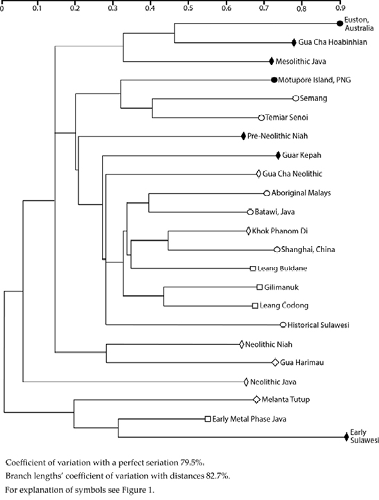
Figure 10.6: Dental metrics, Penrose shape distances, 23 bisexual samples, up to 32 diameters, seriated average-linkage dendrogram.

Sources: Snell 1938; Barrett et al. 1963, 1964; Jacob 1964; Jacob 1967a, 1967b; Doran and Freedman 1974; Brown 1978; Bulbeck 1981; Brace et al. 1984; Tayles 1989; Storm 1995; Bulbeck 2001; Détroit 2002; Bulbeck 2004; Bulbeck 2005a; Bulbeck et al. 2005; Chia et al. 2005; Manser 2005; Noerwidi 2011–12; Bulbeck et al. 2013; this paper.

As shown there, the Early Sulawesi teeth are small (as previously noted by Bulbeck, 2004), smaller than EMP (Leang Codong, Leang Buidane) and historical Sulawesi teeth. The Neolithic Java and Melanta Tutup teeth are small, and the EMP Java teeth are very small. Caution should be exercised in the use of these results, given that they are based on very small sample sizes and incomplete coverage of the dentition. Nonetheless, it is interesting that the late Holocene tooth-size reduction indicated for Java, Borneo and Malaya appears to be reversed for Sulawesi.

Turning to the shape comparisons, we first note that the calibrated shape distances from the third analysis (Table 10.7) were migrated wholesale to the fifth analysis, supplemented here by the calibrated shape distances that involve the four additional samples. As explained in footnote A to Table 10.9, the calibrated shape distances in the fifth analysis vary in terms of the tooth diameters used to generate them, but they are comparable in that the value of 1 serves as the benchmark for the ‘expected’ shape distance in each cell.

Figure 10.6 shows the seriated dendrogram that results from the calibrated shape distances in Tables 10.7 and 10.9. The same general structure emerges as for Figure 10.4. Euston Aborigines, Gua Cha Hoabinhians, Mesolithic Java, Motupore and pre-Neolithic Niah fall towards one pole, while Gua Harimau, Niah Neolithic and historical Sulawesi fall towards the other pole. The four additional samples take up the extreme position at the latter pole. In other words, Neolithic Java, Melanta Tutup, EMP Java and especially Early Sulawesi (but not the Chinese sample) appear particularly non-Australoid. Thus, the Early Sulawesi sample differs from the other mid-Holocene and earlier Indo-Malaysian samples not just by its smaller teeth but also its distinct dental metrical shape.

Discussion

The first assignment for this study was to test the hypothesis that the advent of agriculture and pottery selected for smaller teeth. The expectation required to confirm this hypothesis was evidence for continual tooth-size reduction in Indo-Malaysia throughout the late Holocene. The male comparisons are broadly consistent with this expectation. However, only two late Holocene, prehistoric samples from Indo-Malaysia qualified for inclusion in these comparisons. Further, one of them, Gua Cha Neolithic males, had slightly smaller teeth than Temiar males, even though Temiar ancestry may have included the population represented by the Gua Cha Neolithic burials (Bulbeck, 2011: 237). Certainly, when analysis included the bisexual samples, evidence for continual tooth-size reduction throughout that late Holocene was hard to find. For instance, in the fifth analysis, the Neolithic and recent samples overlap comprehensively in tooth-size, both falling centrally within the EMP range of variation (Figure 10.1e). Similarly, Brace and others (1984) could find no evidence for late Holocene tooth-size reduction in north China, while in mainland Southeast Asia, the Neolithic teeth from Ban Kao in Thailand are smaller than those of recent Thais, and the Iron Age Dong Son teeth smaller than those of recent Vietnamese (Matsumura and Hudson, 2005: Figure 3). Therefore, detailed comparisons appear to falsify the ‘Neolithic tooth-size reduction’ model.

Keeping to a local evolutionary paradigm, we turn to an alternative possible explanation for the tooth-size reduction which characterises Java, Malaya and Borneo, when late Holocene samples are compared with older samples. This explanation, general body-size reduction, is the one preferred by Brown (1989) for the smaller size of Holocene Murray Valley teeth compared to Coobool Creek. It is also Storm’s (1995) proposed explanation for the differences between the Wajak and recent Javanese skulls in their general morphology. However, the available data, sparse as they are, would suggest very large body size in Java right up to the Neolithic (Table 10.10), despite the small teeth as currently documented for Neolithic Java. As for Malaya, Bulbeck (2011) finds evidence for around 10% reduction in stature between the early Holocene and recent times (with reference to the Orang Asli). However, according to Bulbeck’s data, this stature reduction continued throughout the late Holocene, whereas, as shown here, the Gua Cha Neolithic and Gua Harimau teeth appear no larger than those of the Orang Asli. Finally, Zuraina and Pfister (2005) find evidence for a circa 10 cm increase in stature of the Niah Neolithic burials compared to the pre-Neolithic Niah burials. While the small stature estimated for the pre-Neolithic Niah burials (154 cm for males, 145 cm for females) is consistent with the modest size of their teeth, Neolithic Niah appears to combine stature increase with tooth-size reduction. In summary, while a broad correlation between tooth-size and general body size would be expected, general body-size reduction fails as an explanation for late Holocene tooth-size reduction in Borneo, Malaya and Java.

With the falsification of the two mooted, local evolutionary explanations for tooth-size changes in late Holocene Indo-Malaysia, the incursion of ‘new people’ with smaller teeth is left as the default explanation. Although this study was not designed to investigate the source of any such newcomers, the fifth analysis did identify a potential candidate – Early Sulawesi. On the available data, the circa mid-Holocene teeth from Sulawesi are of very typical size by the standards of late Holocene teeth across Indo-Malaysia (Figure 10.1e). The Early Sulawesi teeth also stand at the polar extreme from Australoids in their shape (Figure 10.6), and so would serve as an appropriate precursor for the markedly non-Australoid tooth shape recorded for late Holocene samples from other locations (notably Neolithic and EMP Java, Melanta Tutup, Gua Harimau and Neolithic Niah). The status of Sulawesi as a donor region is reasonable in view of mitochondrial DNA evidence that it was a centre for the dispersal of the E1a, E2a, M7c1c and D5 haplogroups, which together constitute a substantial proportion of recent Indo-Malaysians’ mitochondrial DNA (Hill et al., 2007; Soares et al., 2008).

Table 10.10: Comparative data on major limb-bone lengths(A) in Java.

Specimen/series	Femur length (mm)	Tibia length (mm)	Humerus length (mm)	Source
Wajak (male)	Larger than Hoekgroet	Too fragmentary to assess	Too fragmentary to assess	Storm 1995
Song Terus 1 (Mesolithic male)	470 mm (right)	Not reported	Not reported	Détroit 2002:224
Song Keplek 5 (Neolithic female)	Too fragmentary to assess	390 mm (right)	346 mm (left)	Noerwidi 2011-12
Hoekgroet (Neolithic, female?)	~450 mm	~390 mm	Too fragmentary to assess	Storm 1995
Recent Surabaya males	414.3 + 23.0 (right)	348.0 + 21.0 (right)	296.6 + 16.2 (left)	Bergman and The 1955

Note: A. Femur length in natural position (Martin 2), total tibia length (Martin 1) and maximum humerus length (Martin 1) are the definitions employed by Bergman and The (1955), and also by Noerwidi (2011–12). Détroit (2002) and Storm (1995) do not define their measurements.

Source: All listed in notes section.

At the same time, the evidence relating tooth-size reduction to broader cranial shape is ambiguous, at best. Table 10.11 focuses on the ‘cranial index’ (cranial breadth as a percentage of cranial length) as this is one of the most widely reported observations for prehistoric remains from Indo-Malaysia. The comparison between Wajak and early to mid-Holocene Indo-Malaysians suggests a transition to smaller teeth associated with more elongated, not broader, crania. Late Holocene Indo-Malaysians, for their part, can generally be distinguished from early to mid-Holocene Indo-Malaysians both by their smaller teeth and their broader crania. However, there are exceptions, such as the Puger skull (EMP Java), which combines a narrow braincase with very small teeth.

The dental metrical results outlined here are at variance with recently presented results on the same burial series. Manser (2005) was unable to distinguish between the pre-Neolithic and Neolithic Niah remains on their facial shape, cranial non-metric traits and dental morphology, finding that both resemble recent Southeast Asians, Polynesians and Australian Aborigines. Here, however, we find that the Neolithic teeth from Niah are not only smaller than the pre-Neolithic teeth, as noted by Manser (2005), but also different in shape. As for Gua Cha, Bulbeck (2005a) supported earlier findings of population continuity between the Hoabinhian and Neolithic series, consistent with the decision by Matsumura and Hudson (2004) to pool them into a single ‘Gua Cha’ sample. However, tooth shape analysis would be compatible with a scenario in which the Gua Cha Neolithic burials reflect admixture between the Gua Cha Hoabinhians and Neolithic immigrants from the north, as represented by Khok Phanom Di (Figures 10.4 to 10.6; cf. Bellwood, 1993). Finally, the Java Mesolithic burials appear to be more homogeneous in their cranial shape (Table 10.11) and their dental metrics, and more distinct from the Java Neolithic burials, than Détroit (2002) inferred – although this discrepancy may reflect Détroit’s reliance on a now superseded, pre-Neolithic dating for the critical Song Keplek 5 burial.

Table 10.11: Comparison of Indo-Malaysian tooth-size and cranial index.

Location/Age	Series/specimen	Tooth size(A)	Cranial index(B)	Cranial index data source
Java, Late Pleistocene	Wajak	Very large	Mesocranic (75.5)	Storm 1995
Java, Pleistocene/ Holocene junction	Gua Braholo	Large	Dolichocranic (70.3, 73.9)	Détroit 2002
Malaya, Early Holocene	Gua Peraling 4	Small	Dolichocranic (74.7)	Bulbeck and Adi 2005
Java, mid-Holocene	Song Keplek 4	Large	Mesocranic (77.8)	Détroit 2002
Java, mid-Holocene	Sampung	Large	Dolichocranic	Jacob 1967a
Malaya, mid-Holocene	Gua Cha Hoabinhian	Large	Dolichocranic (72.8, 73.1)	Bulbeck 2005a
Malaya, mid-Holocene	Guar Kepah	Large	Dolichocranic (63.6)	Jacob 1967a
Sulawesi, mid-Holocene	Leang Buidane Pre-ceramic	Medium (Table 10.4)	Dolichocranic (66.8)	Bulbeck 1981
Java, Neolithic	Song Keplek 5	Medium	Brachycranic	Noerwidi 2011–12
Java, Neolithic	Hoekgroet	Small	Brachycranic (80.5)	Storm 1995
Malaya, Neolithic	Gua Cha Neolithic	Small	Mesocranic (76.0), brachycranic (>80)	Bulbeck 2005a
Sulawesi, EMP	Leang Buidane	Medium	Mesocranic	Bulbeck 1981
Java, EMP	Puger	Very small	Dolichocranic (73.9)	Snell 1938
Sulawesi, Recent	Historical Sulawesi	Small	Brachycranic (80.6)	Pietrusewsky 1981(C)
Malaya, Recent	Semang	Small	Mesocranic	Bulbeck and Lauer 2006
Malaya, Recent	Senoi	Small	Mesocranic	Bulbeck and Lauer 2006
Malaya, Recent	Aboriginal Malays	Small	Mesocranic	Bulbeck and Lauer 2006
Java, Recent	Surabaya, Batawi	Small to very small	Brachycranic (81.0)	Pietrusewsky 1981(C)

Notes: A. Tooth-size from this paper except for Gua Peraling 4, from Bulbeck and Adi (2005), and Song Keplek 5, from Noerwidi (2011–12).

B. A cranial index below 75 corresponds to narrow braincases (dolichocrany), while a cranial index above 80 corresponds to broad braincases (brachycrany). Mesocrany (cranial index between 75 and 80) is intermediate.

C. Calculated from the male means for maximum cranial length and cranial breadth.

Sources: Snell 1938; Jacob 1964; Jacob 1967a; Bulbeck 1981; Pietrusewsky 1981; Storm 1995; Détroit 2002; Bulbeck 2004; Bulbeck 2005a; Bulbeck and Adi 2005; Bulbeck et al. 2005; Bulbeck and Lauer 2006; Noerwidi 2011–12; Bulbeck et al. 2013; this paper.

Détroit (2002) hypothesised that Indo-Malaysia was a region of population movements, from the terminal Pleistocene onwards, with links to what is now mainland East Asia to the north and New Guinea (and the Northern Territory) to the southeast. The population history of Indo-Malaysians was more of a swirl in all directions of the compass than a two-layer sequence involving indigenous Australoid foragers and immigrant Neolithic farmers. This hypothesis is consistent with Sulawesi’s possible status as a source for the small teeth and non-Australoid tooth shape found widely across late Holocene Indo-Malaysia. Détroit’s hypothesis is also consistent with the mtDNA findings of Martin Richards and his associates. These findings include significant population movements from Taiwan into Indonesia and from Mainland Southeast Asia into Malaya associated with the introduction of the Neolithic, but also numerous other dispersals into, within and out from Indo-Malaysia’s ‘entangled bank’ (Hill et al., 2007; Soares et al., 2008; Soares et al., 2011; Bulbeck, 2011).

Colin Groves (1976, 1980) developed a strong interest in the macaques and other mammals of Sulawesi, which he explored in the context of both the natural (Groves, 1984) and human-mediated (Groves, 1985, 1995) dispersal of mammals across Indo-Malaysia. Of particular relevance to this paper are his proposals for a sea-borne dispersal of early dogs through Indonesia into New Guinea, and the eastward transport of the Sulawesi warty pig (Sus celebensis) as a domesticate or game animal, prior to the introduction of the dog and pig breeds that could be reasonably associated with the late Holocene migration of Austronesian speakers from Taiwan to Indo-Malaysia. Without reviewing the considerable information now available for human-mediated dispersals of mammals across Indo-Malaysia, we can note that it broadly justifies and indeed extends Colin’s open-minded, exploratory perspective on this topic. Colin taught his students to follow the evidence wherever it leads, an approach which this contribution hopefully illustrates.

Conclusion

Analysis of dental metrical data from Indo-Malaysia suggests a three-stage sequence: very large teeth in the Late Pleistocene; large teeth (except for Sulawesi) between the terminal Pleistocene and mid-Holocene; and small teeth during the late Holocene. Evidence for tooth-size reduction between the Neolithic and recent times was hard to find. This falsifies the model that attributes the small size of late Holocene teeth in Indo-Malaysia to changed selection pressures associated with agriculture and cooking in pots. Also, body-size reduction fails as an explanation for late Holocene tooth-size reduction in Borneo, Java and Malaya. Thus, the change appears to reflect the influx of newcomers, whose teeth were not only smaller than those of their mid-Holocene counterparts but also different in ‘shape’. Although the study was not designed to investigate the origins of these newcomers, mid-Holocene Sulawesi emerged as a possibility, admittedly based on a small sample with incomplete coverage of the dentition.

Acknowledgements

The author’s data collection from Sulawesi skulls in museums was funded by a large Australian Research Council grant to the author and Colin Groves for the ‘Contribution of South Asia to the Peopling of Australasia’ project. The author’s study of teeth from Lake Towuti in Sulawesi was funded by a large Australian Research Council grant (DP 110101357) to Sue O’Connor, Jack Fenner, Janelle Stevenson (Australian National University) and Ben Marwick (University of Washington). The author thanks Marc Oxenham and an anonymous reviewer for their comments on this paper.

References

Anggraeni. 1999. The introduction of metallurgy to Indonesia. MA thesis, The Australian National University. Available from: ANU Library.

Barrett MJ, Brown T, Arato G, Ozols IV. 1964. Dental observations on Australian Aborigines: Buccolingual crown diameters of deciduous and permanent teeth. Aust Dent J 9:280–285.

Barrett MJ, Brown T, MacDonald MR. 1963. Dental observations on Australian Aborigines: Mesiodistal crown diameters of permanent teeth. Aust Dent J 8:150–155.

Bellwood P. 1976. Archaeological research in Minahasa and the Talaud Islands, northeastern Indonesia. AP 19:240–288.

Bellwood P. 1978. Man’s conquest of the Pacific. Sydney: Collins.

Bellwood P. 1993. Cultural and biological differentiation in Peninsular Malaysia: The last 10,000 years. AP 32:37–60.

Bellwood P. 1997. Prehistory of the Indo-Malaysian Archipelago. Revised edition. Honolulu: University of Hawai’i Press.

Bergman RAM, The TH. 1955. The length of the body and long bones of the Javanese. Doc Med Geogr Trop 7:197–214.

Brace CL. 1976. Tooth reduction in the Orient. AP 19:203–219.

Brace CL, Hinton RJ. 1981. Oceanic tooth-size variation as a reflection of biological and cultural mixing. Curr Anthropol 22:549–659.

Brace CL, Shao X-q, Zhang Z-b. 1984. Prehistoric and modern tooth-size in China. In: Smith FH, Spencer, F, editors. The origins of modern humans: A world survey of the fossil evidence. New York, NY: Alan R. Liss. pp. 485–516.

Brown PJ. 1978. The ultrastructure of dental abrasion: Its relationship to diet. BA Hons thesis, The Australian National University.

Brown P. 1981. Sex determination of Aboriginal crania from the Murray River Valley: A reassessment of the Larnach and Freedman technique. Archaeol Ocean 16:53–63.

Brown P. 1989. Coobool Creek. Terra Australis 13. Canberra: The Australian National University.

Bulbeck FD. 1981. Continuities in Southeast Asian evolution since the Late Pleistocene. Some new material described and some old questions reviewed. MA thesis, The Australian National University. Available from: ANU Library.

Bulbeck FD. 1982. A re-evaluation of possible evolutionary processes in Southeast Asia since the late Pleistocene. Bull Indo Pac Pre hi 3:1–21.

Bulbeck D. 1996–97. The Bronze-Iron Age of South Sulawesi, Indonesia: <ortuary traditions, metallurgy and trade. In: Bulbeck FD, Barnard N, editors. Ancient Chinese and Southeast Asian Bronze Age cultures. Taipei: Southern Materials Center Inc. Vol II, pp. 1007–1076.

Bulbeck D. 2001. Human remains from Gua Harimau, West Malaysia. Report to the Department of Museums and Antiquity, Kuala Lumpur, Malaysia. Available from: the author on request.

Bulbeck D. 2004. South Sulawesi in the corridor of island populations along East Asia’s Pacific rim. In: Keates SG, Pasveer JM, editors. Quaternary research in Indonesia. Mod Quat Re 18. Leiden: A.A. Balkema. pp. 221–258.

Bulbeck FD. 2005a. The Gua Cha burials. In: Zuraina M, editor. The Perak Man and other prehistoric skeletons of Malaysia. Penang: Penerbit Universiti Sains Malaysia. pp. 253–309.

Bulbeck D. 2005b. The Guar Kepah human remains. In: Zuraina M, editor. The Perak Man and other prehistoric skeletons of Malaysia. Penang: Penerbit Universiti Sains Malaysia. pp. 383–423.

Bulbeck D. 2011. Biological and cultural evolution in the population and culture history of Malaya’s anatomically modern inhabitants. In: Enfield N, editor. Dynamics of human diversity: The case of Mainland Southeast Asia. Pacific Linguistics 627. Canberra: The Australian National University. pp. 207–255.

Bulbeck D, Adi T. 2005. A description and analysis of the Gua Peraling human remains. In: Zuraina M, editor. The Perak Man and other prehistoric skeletons of Malaysia. Penang: Penerbit Universiti Sains Malaysia. pp. 311–343.

Bulbeck D, Kadir RA, Lauer A, Zamri R, Rayner D. 2005. Tooth-sizes in the Malay Peninsula past and present: Insights into the time depth of the indigenous inhabitants’ adaptations. Int J Indigen Res 1:41–50.

Bulbeck D, Lauer A. 2006. Human variation and evolution in Holocene Peninsular Malaysia. In: Oxenham M, Tayles N, editors. Bioarchaeology of Southeast Asia. Cambridge: Cambridge University Press. pp. 133–171.

Bulbeck D, Marwick B, O’Connor S et al. 2013. Archaeology of Lake Towuti: Survey and excavation in South Sulawesi. Poster presented at the Society of American Archaeology Annual Meeting, 3–7 April, Honolulu, Hawaii.

Carlson DS, Van Gerven DP. 1977. Masticatory function and post-Pleistocene evolution in Nubia. Am J Phys Anthropol 46:495–506.

Chia S. 2008. Prehistoric sites and research in Semporna, Sabah, Malaysia. Bulletin of the Society for East Asian Archaeology 2, www.seaa-web.org/bulletin2008/bul-essay-08-01.htm.

Chia S, Arif J, Matsumura H. 2005. Dental characteristics of prehistoric human teeth from Melanta Tutup, Sabah. In: Zuraina M, editor. The Perak Man and other prehistoric skeletons of Malaysia. Penang: Penerbit Universiti Sains Malaysia. pp. 239–251.

Demeter F. 2006. New perspectives on the peopling of Southeast and East Asia during the late Upper Pleistocene. In: Oxenham M, Tayles N, editors. Bioarchaeology of Southeast Asia. Cambridge: Cambridge University Press. pp. 112–132.

Détroit F. 2002. Origine et evolution des Homo sapiens in Asie du Sud-Est: Descriptions et analyses morphométriques de nouveaux fossils. PhD thesis, Museum National d’Histoire Naturelle. Available from: www.dsifilex.mnhn.fr/get?k=5ZIu9om0ReQJidRUlY9.

Doran GA, Freedman L. 1974. Metrical features of the dentition and arches of populations from Goroka and Lufa, Papua New Guinea. Hum Biol 3:583–594.

Groves CP. 1976. The origin of mammalian fauna of Sulawesi (Celebes). Z Säugetierk 41:201–216.

Groves CP. 1980. Speciation in Macaca: The view from Celebes. In: Lindberg D, editor. The macaques: Studies in ecology, behavior and evolution. New York: Van Nostrand Reinhold. pp. 84–124.

Groves CP. 1984. Mammal faunas and palaeogeography of the Indo-Australian region. Cour Forsch Inst Senckenberg 69:267–273.

Groves CP. 1985. On the agriotypes of domestic cattle and pigs in the Indo-Pacific region. In: Misra VN, Bellwood P, editors. Recent advances in Indo-Pacific prehistory. Leiden: EJ Brill. pp. 429–438.

Groves CP. 1989. A regional approach to the problem of the origin of modern humans in Australasia. In: Mellars P, Stringer C, editors. The human revolution: Behavioural and biological perspectives on the origins of modern humans. Princeton: Princeton University Press. pp. 274–285.

Groves CP. 1995. Domesticated and commensal mammals of Austronesia and their histories. In: Bellwood P, Fox JJ, Tryon D, editors. The Austronesians: Historical and comparative perspectives. Canberra: The Australian National University. pp. 161–173.

Hanihara T. 1994. Craniofacial continuity and discontinuity of Far Easterners in the late Pleistocene and Holocene. J Hum Evol 27:417–441.

Hill C, Soares P, Mormina M, et al. 2007. A mitochondrial stratigraphy for Island Southeast Asia. Am J Hum Genet 80:29–43.

Howells WW. 1973. The Pacific Islanders. London: Weidenfeld & Nicolson.

Jacob T. 1964. A human mandible from the Anjar urn field, Indonesia. J Natl Med Assoc 56:421–426.

Jacob T. 1967a. Some problems pertaining to the racial history of the Indonesian region. Utrecht: Netherlands Bureau for Technical Assistance.

Jacob T. 1967b. Racial identification of the Bronze Age human dentitions from Bali, Indonesia. J Dent Res 46:903–910.

Joliffe IT. 2002. Principal components analysis. Second edition. New York, NY: Springer.

Manser JM. 2005. Morphological analysis of the human burial series at Niah Cave. PhD thesis. Available from: UMI Dissertation Services, Ann Arbor, MI.

Matsumura H, Hudson MJ. 2005. Dental perspectives on the population history of Southeast Asia. Am J Phys Anthropol 127:182–209.

Noerwidi S. 2011–12. The significance of the Holocene human skeleton Song Keplek in the history of human colonization of Java: A comprehensive morphological and morphometric study. MA thesis, Museum National d’Histoire Naturelle. Available from: www.hopsea.mnhn.fr/pc/thesis/M2Noerwidi_5.pdf.

Pardoe C. 1988. The cemetery as symbol: The distribution of prehistoric Aboriginal burial grounds in southeastern Australia. Archaeol Ocean 23:1–16.

Penrose LS. 1954. Distance, size and shape. Ann Eugen 18:337–343.

Pietrusewsky M. 1981. Cranial variation in Early Metal Age Thailand and Southeast Asia studied by multivariate procedures. Homo 32:1–26.

Pietrusewsky M. 2006. A multivariate craniometric study of the prehistoric and modern inhabitants of Southeast Asia, East Asia and surrounding regions: A human kaleidoscope? In: Oxenham M, Tayles N, editors. Bioarchaeology of Southeast Asia. Cambridge: Cambridge University Press. pp. 59–90.

Snell CARD. 1938. Meschelijke skeletresten uit de duin formatie van Java’s zudkust nabij Poeger (Z. Banjoewangi). Surabaya: G. Kolff.

Soares P et al. 2008. Climate change and post-glacial human dispersals in Southeast Asia. Mol Biol Evol 25:1209–1218.

Soares P et al. 2011. Ancient voyaging and Polynesian origins. Am J Hum Genet 88:239–247.

Storm P. 1995. The evolutionary significance of the Wajak skulls. Scripta Geol 110.

Storm P et al. In press. U-series and radiocarbon analyses of human and faunal remains from Wajak. J Hum Evol.

Tayles NG. 1999. The excavation of Khok Phanom Di: A prehistoric Site in Central Thailand. Volume V: The people. London: The Society of Antiquaries.

Tieng FS. 2010. Hoabinhian rocks: An examination of Guar Kepah artifacts from the Heritage Conservation Centre in Jurong. MA thesis, National University of Singapore. Available from: www.scholarbank.nus.edu.sg/bitstream/handle/10635/20404/FooST.pdf?sequence=1.

Turner CG II. 1983. Sundadonty and Sinodonty: A dental anthropological view of Mongoloid microevolution, origin, and dispersal into the Pacific basin, Siberia and the Americas. In: Vasilievsky RS, editor. Late Pleistocene and early Holocene cultural connections of Asia and America. Novosibirsk: USSR Academy of Sciences, Siberian Branch. pp. 147–157.

Zuraina M, Pfister L-A. 2005. The Niah collection of 122 skeletons at the University of Nevada. In: Zuraina M, editor. The Perak Man and other prehistoric skeletons of Malaysia. Penang: Penerbit Universiti Sains Malaysia. pp. 155–173.