6. Educating ‘the Masses’ in China: Unequal Opportunities and Unequal Outcomes

Jane Golley and Sherry Tao Kong

Introduction

Following a staggering growth rate of 10 per cent per annum between 1979 and 2010, China’s growth has steadily decelerated over the past five years, from 7.9 per cent in 2012 to 6.7 per cent in 2016. Yet it remains by far the fastest-growing major economy in the world. In the decades ahead, China aims to sustain its progress of development and to advance from middle-income to high-income status by mid-century. The road towards this ambitious goal is mapped out by a comprehensive reform plan, geared towards switching from a reliance on an abundance of cheap labour to a more innovative, skilled workforce. The success of this transition will require concerted effort on various fronts, among which significant improvements in human capital will be critical.

Compared with the high-income-country group that China aspires to join, the education level of China’s current labour force is shockingly poor. As of 2010, the share of China’s labour force that had ever attended senior high school (24 per cent) is less than one-third of the average upper secondary attainment rate in Organisation for Economic Co-operation and Development (OECD) countries (Khor et al. 2016). Moreover, as this chapter will demonstrate, there is a substantial degree of inequality of educational opportunity across China’s cities and countryside, as well as across a number of other dimensions. While successive generations of Chinese children are better educated than their parents, these unequal opportunities will constrain the country’s human capital potential in the decades ahead.

Inequality of opportunity in education (or in any other measure of economic ‘advantage’) is quite distinct from inequality in educational outcomes. In particular, while there is no clear consensus as to what constitutes the ‘optimal’ or ‘ideal’ level of inequality in outcomes, there is broad consensus that inequality resulting from unequal ‘effort’ is ethically acceptable, while inequality resulting from unequal ‘circumstances’ or opportunities—which lie beyond the control of an individual—is not.

A rapidly growing literature has used this idea as the basis for measuring the extent of inequality of opportunity for a range of economic outcomes—including per capita income, earnings, wealth, consumption and health—in a wide range of countries, confirming that the ideal of equality of opportunity is by far the exception, not the rule. Ferreira and Gignoux (2011), for example, in their analysis of six Latin American countries, find that the share of inequality of opportunity in outcome inequality is substantial, ranging from 23 per cent in Colombia to 34 per cent in Guatemala for household per capita income. Zhang and Eriksson (2010) likewise find a very high share of inequality of opportunity in individual income inequality in China—increasing steadily from 46 per cent in 1989 to 63 per cent in 2006. These papers identify a range of ‘circumstances’ that contribute to inequality of opportunity, with one’s place of birth, gender and parental education levels almost always playing significant roles.

In this chapter, we take it as given that equality of opportunity—as opposed to equality of outcomes—has indisputable merit, and set out to examine the extent to which the educational outcomes of Chinese citizens born between 1940 and 1989 diverge from this ideal. For a country intent on raising the level of human capital to support productivity, growth and a higher value-added economy in the future, equality of opportunity seems like a very good place to start.

The next section introduces the methodology used to calculate inequality of opportunity and identifies the set of ‘circumstance’ variables that we use to measure this in the case of China’s educational attainment (measured in years of schooling), using the China Family Panel Studies (CFPS) surveys for 2010 and 2012. The following section confirms the importance of these variables using regressions for the nationwide sample, and separately for the urban and rural samples, as a way of assessing the unequal opportunities not only between urban and rural populations, but also within them. We then present the key empirical results regarding inequality of opportunity in education in China, before concluding with some policy implications.

Measuring ‘inequality of opportunity’

Method

Attempts to measure ‘inequality of opportunity’ begin with the premise that the observed inequality in any particular economic outcome can be attributed to two components. The first component derives from the different circumstances in which individuals find themselves and over which they have no control—for example, their gender, place of birth or the socioeconomic status of their parents. The second derives from the different levels of effort that individuals may exert to influence a given outcome—for example, how hard they study. This distinction has long been recognised as critical for assessing the extent to which equal opportunity does or does not prevail.

In his seminal paper, Roemer (1998) defines equality of opportunity as a situation in which the distribution of a given outcome is independent of circumstances or, in other words, that all individuals who exert the same effort would achieve the same outcome, regardless of their circumstances. Partitioning the population into groups or ‘types’ of people with identical circumstances and measuring the extent to which this condition is not satisfied provide one measure of inequality of opportunity. An alternative, weaker criterion for equality of opportunity is that the mean outcome levels—rather than the entire distributions—are identical across types, as proposed by Van de Gaer (1993). This criterion involves suppressing ‘intra-type’ inequality and calculating the extent of ‘between-type’ inequality based on the mean levels for each type as a measure of inequality of opportunity.

These ideas have been developed and applied in a burgeoning empirical literature that adopts a range of methods to measure the degree of inequality of opportunity in a range of countries and for a range of different outcomes.¹ Here, we follow the methodology of Ferreira and Gignoux (2011), which has emerged as the most common approach,² adapting it to suit our economic advantage of interest: years of education.

In particular, we begin with a stylised model of advantage (here, years of schooling) of the form y = f(C, E, u), where C is a vector of circumstance variables, E is a vector of effort variables and u represents random unobserved variables. While circumstances are exogenous by definition (that is, they cannot be influenced by any actions of the individual), it is likely that effort will be influenced by a range of factors, including circumstances.³ This implies that the model is more accurately expressed as y = f(C, E(C, v), u). For a number of reasons, touched on further below (and expanded on at length in Ferreira and Gignoux 2011), we choose to treat effort as unobserved and estimate the reduced-form regression (Equation 6.1).

Equation 6.1

y_i = βC_i + ε

In Equation 6.1, y_i is the years of schooling attained by individual i, and C_i is a vector of discrete circumstance variables pertaining to that individual, which allows a partition into types as described above. For example, if there were just two circumstance variables—gender and hukou (household registration) status—there would be a total of four ‘types’: rural boys, rural girls, urban boys and urban girls. Using the estimated coefficients, , and the actual values of circumstances, we construct a distribution, , in which . That is, y is replaced with its prediction, given the vector of circumstances, which is identical for all individuals in any given type, thus eliminating all intra-group inequality. This gives us an absolute scalar measure of inequality of opportunity, . The corresponding relative measure, , determines inequality of opportunity as a share of total inequality, for an appropriate inequality measure, I.

Only certain indexes of inequality satisfy the critical property of additive decomposability that enables total inequality to be decomposed into its between-type and intra-type components—including the generalised entropy class, but not the Gini coefficient. Neither GE(0) (mean log deviation) nor GE(1) (the Theil entropy index) is an option for measuring inequality in educational outcomes as they both involve log values and there are many individuals with no years of schooling (which is not the case in the more standard analyses focused on earnings or consumption). This leaves GE(2), half the coefficient of variation, as the best scalar measure of inequality, which we use below.

We are also interested in the partial contributions of each of the circumstance variables. To assess these, we produce a counterfactual distribution, , where , which assigns the mean level of circumstance J to all individuals, one circumstance at a time. Note that the corresponding partial measures of both the absolute and the relative inequality of opportunity—the latter being —will be lower for a variable that has a larger impact on inequality of opportunity. That is, by eliminating the variation in that variable, inequality of opportunity will fall by a greater amount.

Whatever the number of circumstance variables included in the regression above, an important property of the estimates for IOA and IOR is that they are lower-bound estimates of inequality of opportunity.⁴ This is because the vector of observed circumstances will necessarily be a subset of all relevant circumstances that impact on individual outcomes, with the implication that the estimates for IOA and IOR would be higher if unobserved circumstances were added to the vector C. This lower-bound result, however, applies only to the overall measures of IOA and IOR. In particular, excessive weighting will be attributed to an observable circumstance if it is correlated with an unobservable or omitted one. In this case, will still provide a reasonable measure of all the factors that are linked to the observable circumstances, but it means that the partial estimates, IOR_P, should be treated with caution.

Our decision to treat effort as unobserved is for both practical and logical reasons. We can think of only one variable—hours of study—that could possibly be classified as effort when educational attainment is the outcome of interest, and which is necessarily omitted, as it is not recorded in the survey data utilised below. Whether this is treated as an omitted ‘effort’ variable or an omitted ‘circumstance’ variable, however, the implications are the same. In particular, either it has no correlation with the observed circumstance variables, in which case its omission will not impact on the inequality of opportunity estimates, or it is itself impacted by observed circumstances, in which case this impact will be indirectly incorporated into the estimated coefficients. While this again points to the need for caution in interpreting the regression coefficients as causal links between a given circumstance and the outcome, it is not critical to the measurement of inequality of opportunity, which is the primary concern of this chapter. For a more in-depth discussion on this point, see Golley and Kong (in press).

Which circumstances matter?

Throughout the era of the People’s Republic, China has achieved remarkable advances in expanding its education system and raising the average level of education achieved by its vast population. However, these advances have also resulted in significant educational inequalities along a number of dimensions.

The most prominent dimension of these inequalities is the rural–urban divide, which was solidified by the introduction of the hukou system of household registration in the late 1950s, and which effectively divided—and continues to divide—Chinese citizens into two distinct groups, with starkly different access to China’s expanding education system. An extensive literature has documented the persistent gap in educational attainments between urban and rural China since this time, with weaknesses in the rural education system reflected in higher dropout rates and lower participation at every level of the system, from preschool through to college (see Qiao 2008; Wang et al. 2009; Golley and Kong 2012, 2013; Knight et al. 2012; Yi et al. 2012; Wu 2013; Li et al. 2015).

Another critical dimension of educational inequality in China—and in a large number of other countries as well—stems from intergenerational persistence in educational attainment.⁵ An ongoing debate centres on the extent to which this observed persistence is directly causal (for example, the likelihood that better-educated parents may have greater intellectual capacity because of their own education, rather than because of their innate ability, to invest in educating their children) as opposed to indirectly causal (for example, due to higher genetic intelligence or the greater financial capacity of parents with higher incomes to invest in higher-quality schools) (Black and Devereux 2010). The reason for persistence is not central to the analysis here. Suffice to say that, in its presence, children with better-educated parents find themselves in a relatively enviable circumstance with regard to their prospects, or opportunities, for educational advancement. There is ample evidence to suggest that this is the case in China (see Golley and Kong 2012, 2013; Knight et al. 2012).

The observed persistence in educational attainment across generations feeds into the importance of family origin or socioeconomic status more generally, which has been shown to be of particular significance in China during both the Maoist era (see, for example, Deng and Treiman 1997; Meng and Gregory 2002; Sato and Li 2008) and beyond. A wealth of evidence concurs that during the reform era, the educational advantages of the ‘dominant’ or higher socioeconomic classes—whether measured in terms of parents’ class origins, Communist Party membership, educational levels, occupations or incomes—have been restored and strengthened, with educational inequalities increasing as a result.⁶

The literature reveals a number of other dimensions that have contributed to a widening gap between the most and the least advantaged members of society: across regions, provinces and counties (with children in richer areas achieving higher education levels on average) (Hannum and Wang 2006; Heckmann 2005; Zhang and Kanbur 2005), between different ethnic groups (Hannum 2002) (with Han Chinese maintaining their traditional lead), between genders (Zhang et al. 2007; Zhang and Chen 2014) (with girls being out-educated by boys across all educational levels at nearly all points in time) and between children from families of varying size—invoking Becker and Lewis’s (1973) ‘quantity–quality trade-off’ (see Li et al. 2008; Rosenzweig and Zhang 2009).

Crucially, all the dimensions identified above are essentially ‘circumstances’ into which each individual is born, rather than facing by choice: their hukou status (in childhood), father’s education, parents’ socioeconomic status, province of birth, ethnicity, gender and the number of siblings they have all fall into this category.

We use the CFPS survey, which is a nationally representative biannual longitudinal survey of Chinese communities, families and individuals produced by the Institute of Social Science Survey (ISSS) of Peking University. The CFPS collects individual, family and community-level longitudinal data covering a wide range of economic activities, education outcomes, family dynamics and relationships, migration and health. In the 2010 baseline survey, the CFPS successfully interviewed 14,960 households and 42,590 individuals, with an approximate response rate of 79 per cent. Respondents are tracked through annual follow-up surveys, and we draw on the 2012 survey to take advantage of the supplementary parental information that is missing from the 2010 baseline dataset.

Given the available data, we select the following set of circumstance variables: father’s education level, for which we use three dummy variables—primary school, junior high and senior high and above (with illiteracy as the fourth, excluded category); hukou status at age 12 (urban = 1); gender (male = 1); parents’ Communist Party membership (= 1 if either parent is a member); number of siblings (dummy variables for one or two siblings and three or more siblings, with only children as the third, excluded category); ethnic minority status (= 1 if Han Chinese, 0 for others); and province (with Beijing as the excluded category). To account for the significant variation in educational policies and outcomes over time, we also include dummy variables for each of 10 five-year birth cohorts, from 1940–44 through to 1985–89, before running separate regressions for each of these cohorts. We further investigate the determinants of educational outcomes—and the sources of inequality of opportunity—within the rural and urban subsamples.

Due to data limitations, we do not include parental income or occupation, which, along with education levels, are indicators of socioeconomic status. We also exclude mother’s education level because of the high degree of ‘marriage matching’ observed in China, and hence the high correlation between parents’ education levels (Knight et al. 2012). These variables are hence treated as omitted circumstance variables, which, if correlated with the included variables, will bias their estimated coefficients. This seems most likely for father’s education. While this means we need to be careful interpreting the coefficients on the fathers’ education dummies, it is not problematic for our estimate of inequality of opportunity; it just means that it is a lower-bound result, as discussed above.

Some preliminary statistics for these variables are shown in Table 6.1. This confirms the educational gaps between each of the circumstance variables across the entire national sample, and within the urban and rural samples as well. Not surprisingly, average years of schooling are higher for urban children, boys, Han Chinese, only children and children with parents who are Communist Party members.

One final point worth noting is that our classification of rural or urban based on hukou status ‘at the age of 12’ means that virtually all migrants remain ‘rural’ in the analysis here, with the rural sample accounting for 84 per cent of the total. This is indicative of just how rapid urbanisation has been in recent decades, given a 2013 split of 36–64 per cent for urban and rural hukou holders, respectively, and an even greater share of the population actually living in urban areas, at 54 per cent.

Table 6.1 Preliminary statistics

Education (%)	Nationwide	Urban	Rural
Illiterate	22.7	3.7	26.6
Primary school	20.8	6.0	23.8
Junior high school	32.0	29.4	32.5
Senior high school	13.8	28.5	10.8
College and above	10.8	32.4	6.4
Average schooling (years)	7.4	11.5	6.6
Male (YES = 1, %)	51.3	51.4	51.2
Male average schooling (years)	8.1	11.6	7.4
Female average schooling (years)	6.7	11.4	5.8
Father’s education (%)
Illiterate (no schooling)	44.9	22.3	49.4
Primary school	27.4	26.0	27.7
Junior high school	16.8	23.9	15.4
Senior high school	8.6	18.3	6.6
College and above	2.4	9.6	0.9
Father’s average schooling (years)	4.5	7.3	3.9
Parents party member (YES = 1, %)	12.9	22.2	11.1
Party member average schooling (years)	9.0	12.4	7.7
Non-party member average schooling (years)	7.2	11.2	6.5
Family size (%)
Only child	8.9	23.0	6.0
One or two siblings	40.5	43.2	40.0
Three or more siblings	50.6	33.9	54.0
Only child average schooling (years)	10.0	13.3	7.4
One or two siblings average schooling (years)	8.4	11.7	7.8
Three or more siblings average schooling (years)	6.2	10.1	5.7
Han Chinese (YES = 1, %)	89.3	94.4	88.4
Han average schooling (years)	7.7	11.4	6.9
Minority average schooling (years)	5.4	12.1	4.7
No. of observations	25,937	4,364	21,573

Note: All figures are weighted by CFPS sample weights to be nationally representative.

Sources: CFPS (2010, 2012).

Unequal educational outcomes and their determinants

Before presenting the inequality of opportunity results, this section presents a general picture of trends in educational outcomes across birth cohorts, and their determinants. Figure 6.1 illustrates the rise in average years of schooling attained by successive generations in China, from just 3.9 years for the oldest cohort to 10.1 years for the youngest one nationwide, with children in each cohort being ‘out-educated’ compared with their parents by a large margin. While these average gains are impressive, the figure also shows the persistent gap between the rural and urban populations, peaking at 5.6 years for the 1950–54 cohort and with still a substantial gap of 4.1 years for the youngest cohort.

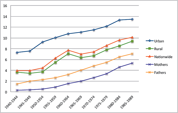
Figure 6.1 Years of schooling across two generations, 1940–89

Sources: CFPS (2010, 2012) and authors’ calculations.

The distributions of educational outcomes for the urban and rural populations are illustrated in Figures 6.2a and 6.2b, respectively. For the urban population, the most striking increase has been at the college level, accounting for just 11 per cent of the 1940–44 cohort compared with 61 per cent of the 1985–89 cohort. The reduction in the urban shares of people either receiving no education (i.e. illiterate) or completing only primary school also stands out, falling from 25 per cent and 24 per cent to 1.7 per cent and 2.1 per cent, respectively, from the oldest to the youngest cohort.

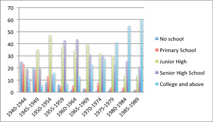
Figure 6.2a Educational attainment, urban China (per cent)

Sources: CFPS (2010, 2012) and authors’ calculations.

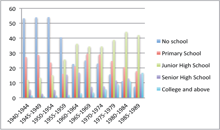
Figure 6.2b Educational attainment, rural China (per cent)

Sources: CFPS (2010, 2012) and authors’ calculations.

For the rural population, the most dramatic change is the reduction in illiteracy, declining from a peak of 54 per cent of the 1945–49 cohort to 7.5 per cent of the youngest cohort. Until the 1960s cohorts, the share of those completing college remained below 4 per cent, increasing substantially since then but still remarkably lower than the equivalent urban share, at just 16.8 per cent for the 1985–89 cohort. As discussed at length in an earlier China Update book (Golley and Kong 2012), the dominant educational attainment in rural China is junior high, remaining at 42 per cent for the youngest cohort.

Table 6.2 presents our chosen measure of inequality in educational outcomes, GE(2), for the national, urban and rural samples (in Column 1) and for each of the 10 five-year cohorts (also illustrated in Figure 6.3). Panel A reveals the overall downward trend in nationwide outcome inequality beginning with the 1945–49 cohort, with the only increase coming between the 1960–64 and 1965–69 cohorts. These trends broadly mirror the rural ones in Panel C—which is to be expected given the dominance of people classified as rural in the sample—and are notably higher than the urban measures for all cohorts. The urban measures in Panel B reveal a steady decline through to the 1960–64 cohort, fluctuating at low levels thereafter.

For comparative purposes, Table 6.2 also presents the Gini coefficients as an alternative measure of outcome inequality,⁷ and one that is more easily interpreted. Importantly, the trends across birth cohorts are the same as those for GE(2) in all three panels, and the values for the rural sample are consistently and substantially higher than those for the urban sample, with values lying between 0.09 for the youngest urban cohort and 0.59 for the 1945–49 rural cohort. The key point here is that the distributions of rural and urban educational outcomes—whether described in terms of the population shares in each education level or summarised as a scalar inequality measure—are significantly different from each other and vary substantially across birth cohorts.

A further point worth noting is that while lower inequality in the urban sample is coupled with higher educational outcomes, this need not necessarily be the case. For example, a Gini of zero would be recorded if all individuals had identical educational outcomes, whether that was illiteracy or college-level education, while if one individual held a PhD, or indeed any positive level of schooling, and the rest of the population was illiterate, the Gini would be one. In this sense, it is impossible to say categorically that any particular level of outcome inequality is better or worse than another. This is what makes measures of inequality of opportunity so valuable, as they reflect the part of inequality that is, quite simply, unjust.

Table 6.2 Inequality in educational outcomes

Cohort	1940–49	1940–44	1945–49	1950–54	1955–59	1960–64	1965–69	1970–74	1975–79	1980–84	1985–89
Panel A: Nationwide
GE(E)	0.21	0.62	0.59	0.54	0.31	0.16	0.20	0.18	0.13	0.10	1.09
Gini	0.35	0.59	0.57	0.56	0.44	0.30	0.34	0.33	0.28	0.25	0.22
Panel B: Urban
GE(2)	0.05	0.25	0.17	0.08	0.06	0.03	0.04	0.04	0.04	0.03	0.03
Gini	0.17	0.40	0.32	0.21	0.16	0.13	0.15	0.16	0.15	0.13	0.12
Panel C: Rural
GE(2)	0.24	0.66	0.66	0.67	0.39	0.19	0.22	0.21	0.15	0.11	0.09
Gini	0.38	0.60	0.60	0.61	0.49	0.33	0.36	0.35	0.29	0.25	0.23

Sources: CFPS (2010, 2012) and authors’ calculations.

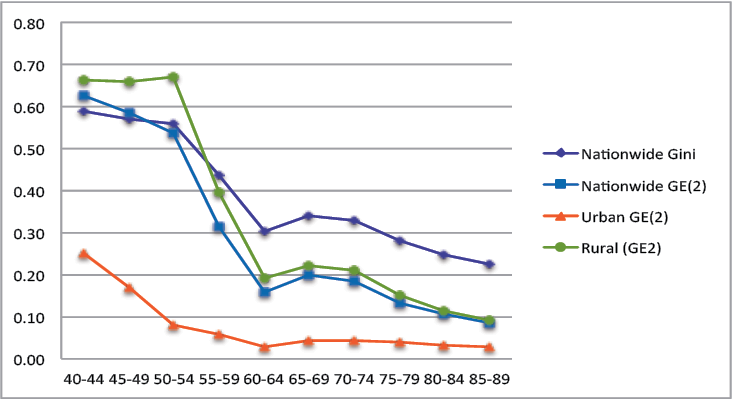
Figure 6.3 Inequality of educational outcomes by cohort

Sources: CFPS (2010, 2012) and authors’ calculations.

Table 6.3 presents the results of the regressions based on Equation 6.1, conducted for the national sample, and separately for the urban and rural samples. Column 1 presents the nationwide results, with all coefficients taking on their expected signs and being highly significant at the 1 per cent level, with the exception of the 1950–54 birth cohort dummy. Most notably, urban hukou status is still associated with an additional three years of schooling (compared with five years in the raw data). It is also clear that better-educated fathers have better-educated children, with primary school, junior high and senior high and above associated with (if not directly causing) an additional 1.6, 2.2 and 3.2 years of schooling, respectively, compared with their illiterate counterparts. Provincial dummies (not reported here for space reasons) are all highly significant and negative, with the exception of Shanghai’s (which is insignificant), with the years of education attained in Beijing exceeding those in Jiangxi, Sichuan and Guizhou by more than three years. The coefficients for the birth cohorts reflect the nationwide trends in educational attainment illustrated in Figure 6.1—generally rising across birth cohorts, with the exception of the 1945–49 and 1965–69 cohorts.

Columns 2 and 3 use the same set of variables (excluding hukou status) for the urban and rural samples, respectively. Most notably, father’s education appears to matter more for rural individuals than for urban ones at every level, peaking at an additional 3.1 years compared with 2.6 years for senior high school and above.

Table 6.3 Determinants of years of schooling: Nationwide, urban and rural

Sample	National	Urban	Rural
Independent variables
Father: Primary school (YES = 1)	1.61***	0.58***	1.70***
Father: Junior high (YES = 1)	2.18***	1.28***	2.29***
Father: Senior high and above (YES = 1)	3.20***	2.71***	3.11***
Hukou at age 12 (Urban = 1)	3.10***
Male (YES = 1)	1.37***	–0.03	1.66***
Parents party member (YES = 1)	0.80***	0.81***	0.78***
One or two siblings (YES = 1)	0.04	–0.56***	0.19
Three or more siblings (YES = 1)	–0.42***	–0.73***	–0.32*
Han Chinese (YES = 1)	0.86***	–0.05	0.94***
Birth cohort:
1945–49	–0.34*	0.23	–0.39*
1950–54	0.03	1.56**	–0.17
1955–59	1.53***	2.33***	1.45***
1960–64	2.89***	3.07***	2.93***
1965–69	2.01***	2.89***	1.90***
1970–74	2.22***	3.25***	2.09***
1975–79	3.03***	3.45***	3.05***
1980–84	3.50***	4.13***	3.42***
1985–89	4.09***	4.31***	4.06***
Provinces	Yes	Yes	Yes
Constant	4.21***	8.85***	5.34***
Observations	23,601	3,775	19,826
R-squared	0.39	0.32	0.31

^*** p < 0.01

^** p < 0.05

^* p < 0.1

Sources: CFPS (2010, 2012) and authors’ own regressions.

Table 6.4 presents the regression results for each birth cohort separately. What is most striking in the nationwide regressions in Panel A is that hukou status is a highly significant determinant of educational outcomes for all cohorts, peaking at 4.5 additional years for urban residents for the 1950–54 cohort and falling to a low of 2.3 years for the youngest cohort. Other interesting points include the declining advantages of being male, to the point of being insignificant for the two youngest cohorts; the consistently positive benefits of having a parent with Communist Party membership; and the significantly negative association of educational attainment with family size for the 1980s cohorts.

Panels B and C reveal some key differences between the urban and rural samples. First, gender clearly matters more in rural areas than urban ones, with the male coefficient insignificant in the latter from the 1960–64 cohort onwards, and even negative for the two youngest cohorts. Second, the schooling advantages associated with parents’ Communist Party membership also differ. For example, for the urban sample, it is insignificant for the 1950s cohorts (the two main Cultural Revolution cohorts), as well as the 1975–79 and 1980–84 cohorts (who would have benefited from the introduction of the compulsory education law in 1986), while it is significant for most rural cohorts apart from the youngest one (possibly reflecting the delayed implementation of the compulsory education law in rural areas). Third, ethnic minority status is significant for the rural sample from the 1970–74 cohort onwards, while for the urban sample it is insignificant throughout.

Finally, the coefficients on the dummies for fathers’ education levels vary substantially across birth cohorts and between the rural and urban samples. For the urban sample, only the senior high school dummy is consistently significant, although notably less so for the oldest cohorts, and reaching a low in magnitude for the 1960–64 cohort—the last of the three cohorts directly impacted by the Cultural Revolution. The coefficient then rises through to the 1975–79 cohort, declining only slightly thereafter but remaining well above those from the pre-reform era, confirming the increasing importance of family socioeconomic status during the reform period. In contrast, for the rural sample, the coefficients on all levels of father’s education tend to be highly significant, with only a few exceptions. Notably, father’s education brings a premium that is greater than for their urban counterparts in all cohorts, suggesting a higher degree of intergenerational persistence.⁸

Table 6.4 Determinants of years of schooling by cohort

Cohort	1940–44	1945–49	1950–54	1955–59	1960–64	1965–69	1970–74	1975–79	1980–84	1985–89
Independent variables
Panel A: Nationwide
Father: Primary school (YES = 1)	2.0***	1.6***	1.4***	1.5***	1.2***	1.8***	1.9***	2.0***	1.5***	1.6***
Father: Junior high (YES = 1)	–0.2	1.2*	0.6	1.6***	1.4***	2.1***	2.5***	2.9***	2.6***	2.3***
Father: Senior high and above (YES = 1)	0.34	2.4***	1.8***	1.2**	3.0***	2.7***	3.8***	4.1***	3.2***	3.7***
Hukou at age 12 (Urban = 1)	2.8***	3.3***	4.5***	3.9***	3.1***	3.5***	3.0***	2.4***	2.6***	2.3***
Male (YES = 1)	3.2***	2.2***	2.8***	3.0***	1.9***	1.5***	1.3***	0.6***	0.1	0
Parents party member (YES = 1)	–0.02	0.5	0.9***	0.6*	0.7***	1.1***	0.6***	0.5***	1.1***	0.9***
One or two siblings (YES = 1)	0.4	–0.1	–0.1	0.7	1.5***	0.7	0.9**	–0.2	–0.8***	–0.7**
Three or more siblings (YES = 1)	0.6	0.1	–0.4	0.6	1.5***	0.4	0.1	–0.8**	–2.3	–2.1***
Han Chinese (YES = 1)	0.1	–0.1	0.3	–0.1	0.9*	–0.1	1.3***	1.2***	1.5***	1.0***
Provinces	Yes	Yes	Yes	Yes	Yes	Yes	Yes	Yes	Yes	Yes
Constant	6.91**	5.0***	4.2***	2.9**	5.5***	5.4***	6.0***	6.7***	8.6***	9.0***
Observations	1,108	1,757	2,451	2,389	2,753	3,268	3,158	2,328	2,079	2,310
R-squared	0.31	0.2	0.3	0.3	0.3	0.3	0.3	0.4	0.4	0.3
Panel B: Urban
Father: Primary school (YES = 1)	1.4	2.3**	0.8	0.6	0.3	–0.2	1.1**	–0.3	0.2	1.6
Father: Junior high (YES = 1)	0.6	1.8	1.9**	1.3	0.3	0.4	1.0*	1.3*	2.4**	2.4
Father: Senior high and above (YES = 1)	0.6	2.0	2.0**	1.8**	1.4***	1.6***	3.6***	3.3***	3.2***	3.9***
Male (YES = 1)	–0.3	1.0	1.0**	0.7	0.2	0.2	0	0	–0.8**	–1.2***
Parents party member (YES = 1)	11.3***	1.1	0.5	0.1	0.3	1.2***	0.9***	0	1.0**	0.7
One or two siblings (YES = 1)	1.4	–0.3	–0.9	–0.5	1.6***	–0.7	–1.0	–0.2	–1.3***	–0.7*
Three or more siblings (YES = 1)	–0.3	0.4	0.3	–1.2	1.0*	–0.9	–1.5**	–0.6	–3.7***	–0.8
Han Chinese (YES = 1)	–2.9	–2.2	–0.4	3.6	–0.6	0.9	–0.5	1.0	0.1	–0.8
Provinces	Yes	Yes	Yes	Yes	Yes	Yes	Yes	Yes	Yes	Yes
Constant	11.3***	9.0***	9.6***	6.2*	11.3***	10.6***	12.8***	11.7***	12.9***	13.4***
Observations	103	242	393	432	466	400	452	403	453	431
R-squared	0.7	0.4	0.2	0.2	0.2	0.2	0.3	0.3	0.3	0.3
Panel C: Rural
Father: Primary school (YES = 1)	2.0***	1.6***	1.5***	1.7***	1.4***	1.9***	1.9***	2.1***	1.5***	1.4***
Father: Junior high (YES = 1)	–0.7	0.9	0.5	1.5***	1.6***	2.3***	2.8***	3.0***	2.7***	2.0***
Father: Senior high and above (YES = 1)	0	2.5***	1.2	0.3	3.3***	2.7***	3.4***	3.8***	2.9***	3.4***
Male (YES = 1)	3.3***	2.3***	3.1***	3.4***	2.4***	1.6***	1.5***	0.7***	0.5**	0.2
Parents party member (YES = 1)	–0.3	0.4	1.1***	0.6*	0.9***	1.1***	0.5*	0.6*	1.0***	1.1**
One or two siblings (YES = 1)	0.3	0.2	0	1.2**	1.8***	1.0*	1.7***	–0.3	–0.5	–0.7**
Three or more siblings (YES = 1)	0.5	0.2	–0.5	1.1**	1.9***	0.8	0.9	–0.8*	–1.8***	–2.2***
Han Chinese (YES = 1)	0	0.1	0.3	–0.2	0.9*	–0.2	1.5***	1.1***	1.8***	1.3***
Provinces	Yes	Yes	Yes	Yes	Yes	Yes	Yes	Yes	Yes	Yes
Constant	14.5***	7.8***	6.0***	8.3***	4.8***	6.0***	6.0***	6.1***	9.5***	9.7***
Observations	1,005	1,515	2,058	1,957	2,287	2,868	2,706	1,925	1,626	1,879
R-squared	0.3	0.2	0.2	0.2	0.2	0.2	0.2	0.3	0.3	0.2

^*** p < 0.01

^** p < 0.05

^* p < 0.1

Note: Standard errors supressed for space reasons.

Sources: CFPS (2010, 2012) and authors’ own regressions.

Inequality of opportunity

Using the regressions reported in Tables 6.3 and 6.4, and the method described above, Table 6.5 presents measures of both the absolute and the relative indexes of inequality of opportunity, IOA and IOR, respectively, along with the inequality of outcome index, GE(2). National trends for these three indexes are illustrated in Figure 6.4, while Figure 6.5 illustrates IOR for the nationwide, urban and rural samples. There are a number of key points.

First, as seen in Figure 6.4, trends in the absolute measure of inequality of opportunity, IOA, are quite distinct from those for inequality of outcomes, GE(2); for some cohorts they move in the same direction, but, for others, the opposite is true. Thus, there is no evidence to suggest that the observed reductions in inequality of outcome have occurred because of an equalising of educational opportunities. More to the point, reductions in inequality of outcome have coincided with increases in inequality of opportunity.

Second, the share of inequality of opportunity in total inequality (IOR) for the nationwide sample fluctuates only slightly for the oldest cohorts, ranging from 24.5 to 32.7 per cent through to the 1965–69 cohort. It is higher than this for every subsequent cohort, peaking at 43.1 per cent of total inequality for the 1980–84 cohort. This confirms that inequality of opportunity has become an increasingly important determinant of unequal educational outcomes during the reform period—and that is not a good sign.

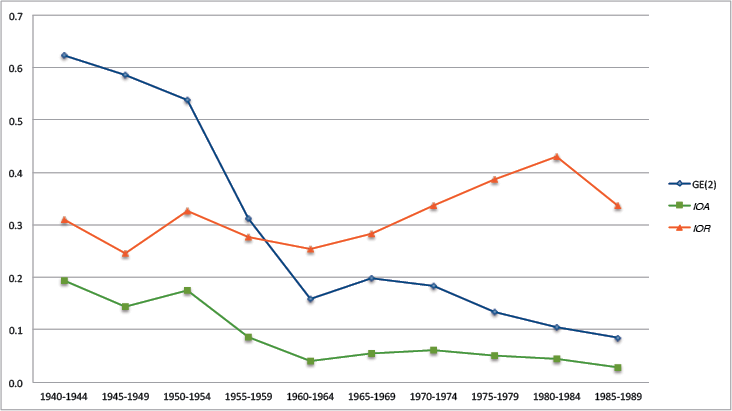
Figure 6.4 Nationwide trends in inequality of outcome and inequality of opportunity

Sources: CFPS (2010, 2012) and authors’ calculations.

Third, as seen in Figure 6.5, trends in the share of inequality of opportunity are quite different in the urban and rural samples—most strikingly, for the three oldest cohorts, but also for the youngest two. The downturn for the youngest rural cohort is a positive sign that opportunities may be improving for the least disadvantaged Chinese children in rural areas. The upturn for the youngest urban cohort is a cause of concern.

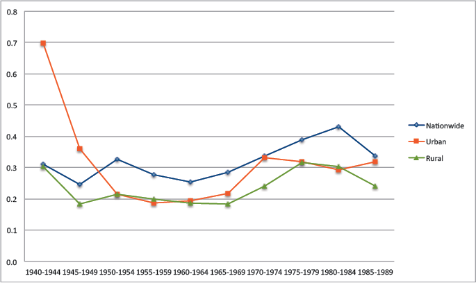
Figure 6.5 Share of inequality of opportunity in inequality of outcome (IOR)

Sources: CFPS (2010, 2012) and authors’ calculations.

And fourth, the nationwide measures of both the absolute and the relative measures of inequality of opportunity in Panel A in Table 6.5 are higher than both the urban and the rural ones from the 1950s onwards (Panels B and C). The reason for this is quite simple: the hukou system, which extends the set of circumstances in the national sample beyond those in the urban and rural samples, clearly creates greater inequality of opportunity in the process.

To push this crucial point further, Table 6.6 presents the partial contributions of each of the circumstance variables. For example, to calculate the partial contribution from hukou status, we assign every individual the ‘average’ value for the dummy variable—that is, equal to the proportion of people with urban hukou, rerun the regressions to generate new predicted values for years of schooling and then calculate the IOR_P associated with these predictions.

The results are ranked in order of importance, revealing that the largest single contributor to inequality of opportunity is hukou status. Both this and father’s education play a stronger role than either one’s province or one’s year of birth, which is quite astounding. Having parents with Communist Party membership ranks above being male, coming from a single-child family or being Han Chinese. Clearly, however, each of these factors plays a role in preventing equality of opportunity from being achieved in China’s educational outcomes.

Table 6.5 Inequality of opportunity: Nationwide, urban and rural

		By birth cohort
	All	1940–44	1945–49	1950–54	1955–59	1960–64	1965–69	1970–74	1975–79	1980–84	1985–89
Panel A: Nationwide
Total (outcome) inequality
GE(2)	0.207	0.624	0.585	0.538	0.313	0.158	0.198	0.185	0.134	0.105	0.085
Inequality of opportunity
Absolute: IOA	0.082	0.194	0.143	0.176	0.086	0.040	0.056	0.062	0.052	0.045	0.029
Relative: IOR	0.393	0.311	0.245	0.327	0.276	0.253	0.284	0.338	0.388	0.431	0.338
Panel B: Urban
Total (outcome) inequality
GE(2)	0.052	0.250	0.170	0.079	0.057	0.030	0.044	0.042	0.041	0.033	0.028
Inequality of opportunity
Absolute: IOA	0.016	0.175	0.061	0.017	0.011	0.006	0.010	0.014	0.013	0.010	0.009
Relative: IOR	0.316	0.700	0.361	0.214	0.187	0.194	0.218	0.331	0.319	0.292	0.319
Panel C: Rural
Total (outcome) inequality
GE(2)	0.238	0.662	0.658	0.671	0.395	0.190	0.221	0.211	0.149	0.113	0.091
Inequality of opportunity
Absolute: IOA	0.073	0.200	0.121	0.144	0.079	0.036	0.040	0.051	0.047	0.034	0.022
Relative: IOR	0.306	0.303	0.184	0.214	0.200	0.187	0.183	0.241	0.317	0.304	0.240

Sources: CFPS (2010, 2012) and authors’ calculations based on regression results in Tables 6.3 and 6.4.

Table 6.6 Partial contributions to relative inequality of opportunity (IOR_P)

			By birth cohort
Circumstance	All		1940–44		1945–49		1950–54		1955–59		1960–64		1965–69		1970–74		1975–79		1980–84		1985–89
Hukou at age 12	0.22	1	0.12	2	0.08	1	0.10	1	0.12	1	0.14	1	0.14	1	0.19	2	0.26	2	0.29	1	0.24	1
Father’s education	0.24	2	0.31	4	0.11	3	0.19	3	0.23	3	0.15	2	0.19	1	0.19	3	0.24	1	0.33	3	0.25	2
Birth year cohort	0.24	3
Province	0.25	4	0.06	1	0.08	2	0.15	2	0.29	6	0.15	3	0.20	3	0.18	1	0.29	3	0.30	2	0.26	3
Parents party member	0.33	5	0.31	5	0.20	5	0.24	5	0.24	4	0.22	5	0.22	4	0.29	5	0.35	4	0.36	4	0.29	4
Male	0.33	6	0.17	3	0.15	4	0.19	4	0.18	2	0.20	4	0.23	5	0.28	4	0.36	6	0.43	6	0.34	6
Number of siblings	0.37	7	0.40	7	0.25	7	0.29	6	0.34	7	0.38	7	0.33	7	0.38	6	0.36	5	0.36	5	0.03	5
Han Chinese	0.49	8	0.33	6	0.24	6	0.37	7	0.27	5	0.32	6	0.28	6	0.47	7	0.51	7	0.58	7	0.41	7

Sources: CFPS (2010, 2012) and authors’ calculations based on regression results in Table 6.4: Panel A.

Conclusions

This chapter investigated trends in educational inequality in China, focusing on the contribution of ‘inequality of opportunity’ to these trends. Utilising the CFPS survey results for 2010 and 2012, we measured the inequality in individual educational outcomes (years of schooling) for the nationwide sample and for separate rural and urban subsamples, in aggregate and for each of 10 birth cohorts. Our regressions identified the key determinants of these outcomes, all of which, we argued, could be classified as ‘circumstances’ that lie beyond the control of each individual, revealing important variations in the magnitude and significance of key determinants across birth cohorts and between the rural and urban subsamples. These results were used to calculate the share of inequality of opportunity in overall educational inequality. The lack of equal opportunity for Chinese citizens with regard to their educational outcomes was shown to stem primarily from the divisive hukou system, with further significant contributions from father’s education level, birth cohort, province, parents’ Communist Party membership, gender, family size and ethnicity, in that order.

Unequal educational attainments across a diverse population—with diverse aptitudes, aspirations and motivations—are to be expected, and there is no sense in which our results suggest this should be otherwise. Rather, what matters is the extent to which these unequal outcomes are determined by factors for which an individual is not responsible and which they cannot change; and there is a very clear case to be made for policies that minimise the impact of these factors and promote equal opportunity for all. The ethical imperative for the ruling Communist Party to address this issue is compounded by the economic importance of finding new sources of growth, particularly in the context of an ageing population and diminishing workforce.

It certainly does not follow that the coefficients on all of the selected circumstance variables should have been insignificantly different from zero. The omission of unobserved variables meant that the estimated coefficients were likely to exhibit some bias and could not be treated as causal. The most obvious of these was the coefficient on father’s education, which likely incorporated not only the omitted impacts of his (and the mother’s) income and occupation, but also reflected some degree of genetic inheritability, which would and should generate inequality in educational outcomes; beyond all others, this coefficient clearly should not be zero.

This point about causality notwithstanding, the results presented in this chapter provide a basis for identifying some reasonable ‘equal opportunity policies’ in China’s education sphere. On the rural–urban gap, hukou system reforms that grant the children of rural migrant workers access to the urban schooling systems where they live are clearly a step in the right direction. Other equalising measures could target a reduction in the private educational costs borne by rural residents who are least able to afford them, such as the liangmian yibu (‘the two waivers, one subsidy’) program that became national law in 2006, and the forbidding of charges and other miscellaneous fees for primary and junior high school. More generally, in a country where intergenerational persistence and educational costs are both on the rise, policies to facilitate the poorest rural children—and, for that matter, the poorest urban children, too—remaining in school for as long as they have the capacity and desire to do so, seem eminently reasonable. Making education accessible and affordable for all should be the number one priority in this regard.

Another set of policy actions relates to the possibility of using affirmative action to address unequal opportunities, by applying different test score standards or admission requirements depending on an individual’s circumstances. This has been a longstanding practice for China’s ethnic minorities (as discussed in Sautman 1999; Yang and Wu 2009), and one that continues to make sense based on our results here, particularly given the concentration of ethnic minorities in the country’s most remote poor rural areas. One practice that makes less sense would be any kind of affirmative action in favour of boys, despite the fact that girls have begun to outperform them in recent years—as evidenced by revelations in 2012 that girls were required to have higher admission scores than boys for entry into the same university courses, a practice that has since been banned. As found in a detailed study by Zhang et al. (2012) on this point, this likely reflects the fact that girls study harder—and they certainly should not be discriminated against because of that.

China has made remarkable progress in advancing the average level of educational attainment during the past seven decades, with considerable expansion of rural education programs in recent times. However, the education gaps between children living in cities and those in villages, in first-tier metropolitan cities such as Beijing and Shanghai and the rest of the country, and from different socioeconomic backgrounds more broadly remain substantial.

To successfully transform into a more technology-based economy capable of long-term sustainable growth, China will require an increasingly skilled labour force. Efforts to ensure that all those children who are most capable, rather than just those who are most fortunate, can access the quality and quantity of education they deserve will raise the likelihood of achieving this development goal. Our results lend quantitative support to the necessity of such an effort.

References

Becker, G. and Lewis, H. (1973), On the interaction between the quantity and quality of children, Journal of Political Economy 81(2): 773–824. doi.org/10.1086/260166.

Black, S. E. and Devereux, P. J. (2010), Recent developments in intergenerational mobility, Handbook of Labor Economics 4(B): 1487–541.

Bourguignon, F., Ferreira, F. and Menendez, M. (2007), Inequality of opportunity in Brazil, Review of Income and Wealth 53(4): 585–618. doi.org/10.1111/j.1475-4991.2007.00247.x.

Brunori, P., Ferreira, F. and Peragine, V. (2013), Inequality of opportunity, income inequality and economic mobility: Some international comparisons, IZA Discussion Paper No. 7155, Institute of Labor Economics, Bonn. Available from: ftp.iza.org/dp7155.pdf. doi.org/10.1596/1813-9450-6304.

Checchi, D. and Peragine, V. (2010), Inequality of opportunity in Italy, Journal of Economic Inequality 8(4): 429–50. doi.org/10.1007/s10888-009-9118-3.

Checchi, D., Fiorio, C. V. and Leonardi, M. (2008), Intergenerational persistence in educational attainment in Italy, Paper presented at 30th General Conference of The International Association for Research in Income and Wealth, Dresden, Germany, August.

Deng, Z. and Treiman, D. J. (1997), The impact of the Cultural Revolution on trends in educational attainment in the People’s Republic of China, The American Journal of Sociology 103(2): 391–428. doi.org/10.1086/231212.

Emran, M. S. and Sun, Y. (2015), Magical transition? Intergenerational educational and occupational mobility in rural China: 1988–2002, Policy Research Working Paper 7316, June, Office of the Chief Economist for East Asia and the Pacific Region, The World Bank, Washington, DC. Available from: documents.worldbank.org/curated/en/229911468000896844/pdf/WPS7316.pdf.

Ferreira, F. and Gignoux, J. (2011), The measurement of inequality of opportunity: Theory and an application to Latin America, Review of Income and Wealth 57(4): 622–57. doi.org/10.1111/j.1475-4991.2011.00467.x.

Golley, J. and Kong, S. T. (2012), Climbing the intergenerational ladder of education in urban, rural and migrant China, in H. Mackay and L. Song (eds), Rebalancing and Sustaining Growth in China, Canberra: ANU E Press.

Golley, J. and Kong, S. T. (2013), Inequality in the intergenerational mobility of education in China, China and the World Economy 21(2): 15–37.

Golley, J. and Kong, S. T. (in press), Inequality of opportunity in China’s educational outcomes, China Economic Review. doi.org/10.1016/j.chieco.2016.07.002.

Hannum, E. (2002), Educational stratification by ethnicity in China: Enrolment and attainment in the early reform years, Demography 39(1): 95–117. doi.org/10.1353/dem.2002.0005.

Hannum, E. and Wang, M. (2006), Geography and educational inequality in China, China Economic Review 17: 253–65. doi.org/10.1016/j.chieco.2006.04.003.

Heckman, J. (2005), China’s human capital investment, China Economic Review 16(1): 50–70. doi.org/10.1016/j.chieco.2004.06.012.

Hertz, T., Jayasundera, T., Piraino, P., Selcuk, S., Smith, N. and Verashchagina, A. (2007), The inheritance of educational inequality: International comparisons and fifty-year trends, The B. E. Journal of Economic Analysis and Policy 7(2): 1–46.

Khor, N., Pang, L., Liu, C., Chang, F., Mo, D., Loyalka, P. and Rozelle, S. (2016), China’s looming human capital crisis: Upper secondary educational attainment rates and the middle-income trap, The China Quarterly 228: 905–26. doi.org/10.1017/S0305741016001119.

Knight, J., Sicular, T. and Yue, X. (2012), Educational inequality in China: The intergenerational dimension, CIBC Working Paper Series No. 2011-13, Centre for Human Capital and Productivity, University of Western Ontario, London.

Lefranc, A., Pistolesi, N. and Trannoy, A. (2008), Inequality of opportunities vs. inequality of outcomes: Are Western societies alike? The Review of Income and Wealth 54(4): 513–46. doi.org/10.1111/j.1475-4991.2008.00289.x.

Li, H., Loyalka, P., Rozelle, S., Wu, B. and Xie, J. (2015), Unequal access to college in China: How far have poor, rural students been left behind? SFI Working Paper Series No. SFIWP0046, Shanghai Finance Institute, Shanghai.

Li, H. J., Zhang J. and Zhu, Y. (2008), The quality–quantity trade-off of children in a developing country: Identification using Chinese twins, Demography 45(1): 223–43. doi.org/10.1353/dem.2008.0006.

Liu, J. (2006), Expansion of higher education in China and inequality in entrance opportunities, [in Chinese], Chinese Journal of Sociology 26(3): 158–79.

Marrero, G. and Rodríguez, J. G. (2012), Inequality of opportunity in Europe, Review of Income and Wealth 58(4): 597–620. doi.org/10.1111/j.1475-4991.2012.00496.x.

Meng, X. and Gregory, R. G. (2002), The impact of interrupted education on subsequent educational attainment: A cost of the Chinese Cultural Revolution, Economic Development and Cultural Change 50(4): 935–59. doi.org/10.1086/342761.

Qiao, J. (2008), Differentiation of entrance opportunity for higher education in urban and rural areas, [in Chinese], Journal of Education Studies 4(5): 92–6.

Roemer, J. (1998), Equality of Opportunity, Cambridge, Mass.: Harvard University Press.

Rosenzweig, M. and Zhang, J. (2009), Do population control policies induce more capital investment? Twins, birth weight and China’s ‘one-child’ policy, Review of Economic Studies 76(3): 1149–74. doi.org/10.1111/j.1467-937X.2009.00563.x.

Sato, H. and Li, S. (2008), Class origin, family culture, and intergenerational correlation of education in rural China, Global COE Hi-Stat Discussion Paper Series 007, Institute of Economic Research, Hitotsubashi University, Tokyo.

Sautman, B. (1999), Expanding access to higher education for China’s national minorities: Policies of preferential admissions, in G. A. Postiglione (ed.), China’s National Minority Education: Culture, schooling and development, pp. 173–210, New York: Falmer Press.

Singh, A. (2012), Inequality of opportunity in earnings and consumption expenditure: The case of Indian men, Review of Income and Wealth 58(1): 79–106. doi.org/10.1111/j.1475-4991.2011.00485.x.

Van de Gaer, D. (1993), Equality of opportunity and investment in human capital, PhD dissertation, Catholic University of Louvain, Louvain-la-Neuve, Belgium.

Wang, X., Liu, C., Zhang, L., Luo, R., Glauben, T., Shi, Y., Rozelle, S. and Sharbono, B. (2009), What is keeping the poor out of college? Enrolment rates, educational barriers and college matriculation in China, REAP Working Paper 210, September, Rural Education Action Program, Stanford University, California.

Wu, X. (2009), Economic transition, school expansion and educational inequality in China, 1990–2000, [in Chinese], Chinese Journal of Sociology 29(5): 88–113.

Wu, Y. (2013), The inequality and evolution of China’s urban–rural educational opportunities, 1978–2008, [in Chinese], China Social Science (3): 4–21.

Yang, R. and Wu, M. (2009), Education for ethnic minorities in China: A policy critique, SA-eDUC Journal 6(2): 117–31.

Yi, H., Zhang, L., Luo, R., Shi, Y., Mo, D., Chen, X., Brinton, C. and Rozelle, S. (2012), Dropping out: Why are students leaving junior high in China’s poor rural areas? International Journal of Educational Development 32: 555–63. doi.org/10.1016/j.ijedudev.2011.09.002.

Zhang, J., Pang, X., Zhang, L., Medina, A. and Rozelle, S. (2012), Gender inequality of education in China: A meta-regression analysis, REAP Working Paper 239, May, Rural Education Action Program, Stanford University, California.

Zhang, X. and Kanbur, R. (2005), Spatial inequality in education and healthcare in China, China Economic Review 16: 189–204.

Zhang, Y. and Eriksson, T. (2010), Inequality of opportunity and income inequality in nine Chinese provinces, 1986–2006, China Economic Review 21(4): 607–16. doi.org/10.1016/j.chieco.2010.06.008.

Zhang, Y., Kao, G. and Hannum, E. (2007), Do mothers in rural China practice gender equality in educational aspirations for their children? Comparative Education Review 51(2): 131–57. doi.org/10.1086/512023.

Zhang, Z. and Chen, Q. (2014), The expansion of higher education admissions and the gender equalization of higher education opportunity: An empirical study based on Chinese General Social Survey (CGSS2008) data, The Journal ofChinese Sociology 1: 1–19. doi.org/10.1186/s40711-014-0001-7.

Zhou, X., Moen, P. and Brandon Tuma, N. (1998), Educational stratification in urban China: 1949–94, Sociology of Education 71(3): 199–222. doi.org/10.2307/2673202.

---